Least-square fitting using matrix derivatives

Vivek Yadav

1. Introduction

Curve fitting refers to fitting a predefined function that relates the independent and dependent variables. The first step in computing the best curve or line is to parameterize the error function using fewer scalar variables, calculate the derivative of the error with respect to the parameters and compute the parameters that minimize the error cost function. Error is chosen as square instead of absolute value because squared value penalizes data away from fitted curve by scaling it up by the magnitude of error, i.e. a deviation of 2 will be recorded as 4. Therefore, minimizing the summed square of errors results in fits that prefer smaller errors. The most common technique to solve for the parameters that specify the curve is to determine the direction of reducing error and take a small step in that direction, and repeat this process until convergence. This process of iteratively solving for the parameters is also refered as gradient descent. We will go over basic matrix calculations, and will apply them to derive the parameters for best curve fits. In certain special cases, where the predictor function is linear in the unknown parameters, a closed form pseudoinverse solution can be obtained. This post presents both gradient descent and pseudoinverse-based solution for calculating the fitting parameters.

2. First order derivatives with respect to a scalar and vector

This section presents the basics of matrix calculus and shows how they are used to express derivatives of simple functions. First, lets clarify some notations, a scalar is represented by a lower case non-bold letter like $a$, a vector by a lower case bold letter such as $ \textbf{a} $ and a matrix by a upper case bold letter $ \mathbf{A} $.

2.1 Derivative of a scalar function with respect to vector

Derivative of a scalar function with respect to a vector is the vector of the derivative of the scalar function with respect to individual components of the vector. Therefore, for a function $f $ of the vector $ \mathbf{x} $,

$\frac{\partial{ f ( \mathbf{x}} ) }{\partial{\mathbf{x}}}= \left[ \frac{\partial{ f ( \mathbf{x}} ) }{\partial{x_1}} \frac{\partial{ f ( \mathbf{x}} ) }{\partial{x_2}} ... \frac{\partial{ f ( \mathbf{x}} ) }{\partial{x_n}} \right]^T$

Similarly, the derivative of the dot product of two vectors $ \mathbf{a} $ and $ \mathbf{x} $ in $ R^n $ can be written as,

$\frac{\partial{ \mathbf{x}^T \mathbf{a}}}{\partial{\mathbf{x}}} = \frac{\partial{ \mathbf{a}^T \mathbf{x}}}{\partial{\mathbf{x}}}= \mathbf{a}$

Similarly,

$\frac{\partial{ \mathbf{A} \mathbf{x}}}{\partial{\mathbf{x}}} = \mathbf{A}$

* NOTE: If the function is scalar, and the vector with respect to which we are calculating the derivative is of dimension $ n \times 1 $ , then the derivative is of dimension $ n \times 1 $.*

2.2 Derivative of a vector function with respect to a scalar

Derivative of a vector function with respect to a scalar is the vector of the derivative of the vector function with respect to the scalar variable. Therefore, for a function $ \mathbf{f} $ of the variable $ x $,

$\frac{\partial{ \mathbf{f (x}} ) }{\partial{x}}= \left[ \frac{\partial{ f_1 ( \mathbf{x}} ) }{\partial{x}} \frac{\partial{ f_2( \mathbf{x}} ) }{\partial{x}} \ldots \frac{\partial{ f_m ( \mathbf{x}} ) }{\partial{x}} \right]^T$

* NOTE: If the function is a vector of dimension $ m \times 1 $ then its derivative with respect to a scalar is of dimension $ m \times 1 $.*

2.3 Derivative of a vector function with respect to vector

Derivative of a vector function with respect to a vector is the matrix whose entries are individual component of the vector function with respect to to individual components of the vector. Therefore, for a vector function $ \mathbf{f} $ of the vector $ \mathbf{x} $,

$\frac{\partial{ \mathbf{ f(x}} ) }{\partial{\mathbf{x}}}= \left[ \frac{\partial{ \mathbf{ f(x)}} }{\partial{x_1}} \frac{\partial{ \mathbf{ f(x)}} }{\partial{x_2}} ... \frac{\partial{ \mathbf{ f(x)}} }{\partial{x_n}} \right]$ $\left( \begin{array}{c} \frac{\partial{ f_1 ( \mathbf{x}} ) }{\partial{\mathbf{x}}} \\ \frac{\partial{ f_2 ( \mathbf{x}} ) }{\partial{\mathbf{x}}} \\ \vdots \\ \frac{\partial{ f_m ( \mathbf{x}} ) }{\partial{\mathbf{x_1}}} \end{array} \right) = \left( \begin{array}{cccc} \frac{\partial{ f_1 ( \mathbf{x}} ) }{\partial{x_1}} & \frac{\partial{ f_1 ( \mathbf{x}} ) }{\partial{x_2}} & \ldots & \frac{\partial{ f_1 ( \mathbf{x}} ) }{\partial{x_n}}\\ \frac{\partial{ f_2 ( \mathbf{x}} ) }{\partial{x_1}} & \frac{\partial{ f_2 ( \mathbf{x}} ) }{\partial{x_2}} & \ldots & \frac{\partial{ f_2 ( \mathbf{x}} ) }{\partial{x_n}}\\ \vdots & \vdots & \ddots & \vdots \\ \frac{\partial{ f_m ( \mathbf{x}} ) }{\partial{x_1}} & \frac{\partial{ f_m ( \mathbf{x}} ) }{\partial{x_2}} & \ldots & \frac{\partial{ f_m ( \mathbf{x}} ) }{\partial{x_n}} \end{array} \right)$

* NOTE: If the function is a vector of dimension $ m \times 1 $, and the vector with respect to which we are calculating the derivative is of dimension $ n \times 1 $, then the derivative is of dimension $ m \times n $ .*

For the special case where,

$\alpha(x) = \mathbf{x^T A x}$ ,

$\frac{\partial \alpha(\mathbf{x})}{ \partial \mathbf{x}} = \mathbf{x^T (A^T+A)}$

3. Application of derivative of a scalar with respect to a vector

One example where the concepts derived above can be applied is line fitting. In line fitting, the goal is to find the vector of weights that minimize the error between the target value and predictions from a linear model.

Problem statement

Given a set of $ N $ training points such that for each $ i \in [0,N] $, $ \mathbf{x}_i \in R^M $ maps to a scalar output $y_i$, the goal is to fine a linear vector $\mathbf{a}$ such that the error

$J \left(\mathbf{a},a_0 \right) = \frac{1}{2} \sum_{i}^{N} \sum_{j}^{m} \left( a_j x_{i,j} + a_0 - y_i \right)^2 ,$

is minimized. Where $a_j $ is the $ j^{th} $ component and $ a_0 $ is the intercept.

Solution

First we will augment the independent vector $ \mathbf{x}_i $ by inserting a new element 1 to the end of it, and we will augment vector $ \mathbf{a} $ by inserting $ a_0 $ at the end. This will result in the cost functin changing as,

$J \left(\mathbf{W} \right) = \frac{1}{2} \sum_{i}^{N} \sum_{j}^{m+1} \left( w_j x_{i,j} - y_i \right)^2 ,$

The cost fuction above can be rewritten as a dot product of the error vector

$e(W) = \left( X W - y \right) .$

where X is a matrix of n times m+1, y is a n-dimensional vector and W is (m+1)-dimensional vector.

Therefore, the cost function J is now, $J \left(\mathbf{W} \right) = \frac{1}{2} e(W)^T e(W)= \frac{1}{2} \left( \mathbf{ X W - y } \right)^T \left(\mathbf{ X W - y } \right) .$

Expanding the transpose term, $J \left(\mathbf{W} \right) = \frac{1}{2} \left( \mathbf{W^T X^T - y^T} \right) \left(\mathbf{ X W - y }\right)$

$= \frac{1}{2} \left( \mathbf{ W^T X^T X W - 2 y^T X W + y^T y} \right)$

Note, all terms in the equation above are scalar. Taking derivative with respect to W gives,

$\frac{\partial \mathbf{J}}{\partial \mathbf{W}} = \left( \mathbf{ W^T X^T X - y^T X } \right)$

Gradient-descent method

Minimum is obtained when the derivative above is zero. Most commonly used approach is a gradient descent based solution where we start with some initial guess for W, and update it as,

$\mathbf{W_{k+1}} = \mathbf{W_{k}} - \mu \frac{\partial \mathbf{J}}{\partial \mathbf{W}}$

It always a good idea to test if the analytically computed derivative is correct, this is done by using the central difference method, $\frac{\partial \mathbf{J}}{\partial \mathbf{W}}_{numerical} \approx \frac{\mathbf{J(W+h) - J(W-h)}}{2h}$

Central difference method is better suited because the central difference method has error of $ O(h^2 $, while the forward difference has error of $ O(h) $. Interested readers may look up Taylor series expansion or may choose to wait for a later post.

Pseudoinverse method

Another method is to directly compute the best solution by setting the first derivative of the cost function to zero.

$\frac{\partial \mathbf{J}}{\partial \mathbf{W}} = \left( \mathbf{ W^T X^T X - y^T X } \right) = \mathbf{0}$

By taking transpose and solving for W,

$\mathbf{W} = \mathbf{ \underbrace{(X^T X)^{-1}X^T}_{Pseudoinverse} ~ y }$

Example: Line fitting

In this part, we will generate some data and apply the methods presented above. We will get the equation of the best fit line using gradient descent and pseudo inverse methods, and compare them.

## Generate toy data
import numpy as np
import matplotlib.pyplot as plt
import time 
%pylab inline

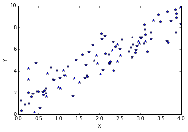
X = 4*np.random.rand(100)
Y = 2*X + 1+ 1*np.random.randn(100)

X_stack = np.vstack((X,np.ones(np.shape(X)))).T

plt.plot(X,Y,'*')
plt.xlabel('X')
plt.ylabel('Y')

Fig1. Noisy data

Line fitting using gradient descent

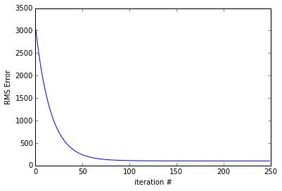
Gradient descent method is used to calculate the best-fit line. A small value of learning rate is used. We will discuss how to choose learning rate in a different post, but for now, lets assume that 0.00005 is a good choice for the learning rate. Gradient is computed using the equation presented in section 2.3, and the weights (or coefficients) are stored for each step.

def get_numerical_derv(W):
    h = 0.00001

    W1 = W + [h,0]
    errpl1 = np.dot(X_stack,W1)-Y
    W1 = W - [h,0]
    errmi1 = np.dot(X_stack,W1)-Y
    W2 = W + [0,h]
    errpl2 = np.dot(X_stack,W2)-Y
    W2 = W - [0,h]
    errmi2 = np.dot(X_stack,W2)-Y
    
    dJdW_num1 = (np.dot(errpl1,errpl1)-np.dot(errmi1,errmi1))/2./h/2.
    dJdW_num2 = (np.dot(errpl2,errpl2)-np.dot(errmi2,errmi2))/2./2./h

    dJdW_num = [dJdW_num1,dJdW_num2]
    return dJdW_num

t0 = time.time()
W_all = []
err_all = []
W = np.zeros((2))
lr = 0.00005
h = 0.0001
for i in np.arange(0,250):
    

    
    W_all.append(W)
    err = np.dot(X_stack,W)-Y
    err_all.append(  np.dot(err,err) )
    XtX = np.dot(X_stack.T,X_stack)
    dJdW = np.dot(W.T,XtX) - np.dot(Y.T,X_stack)
    if (i%50)==0:
        dJdW_n = get_numerical_derv(W)
        print 'Iteration # ',i
        print 'Numerical gradient: [%0.2f,%0.2f]'%(dJdW_n[0],dJdW_n[1])
        print 'Analytical gradient:[%0.2f,%0.2f]'%(dJdW[0],dJdW[1])
    
    W = W - lr*dJdW

tf = time.time()
print 'Gradient descent took %0.6f s'%(tf-t0)

plt.plot(err_all)
plt.xlabel('iteration #')
plt.ylabel('RMS Error')

Iteration #  0
Numerical gradient: [-1255.13,-505.70]
Analytical gradient:[-1255.13,-505.70]
Iteration #  50
Numerical gradient: [-264.16,-115.18]
Analytical gradient:[-264.16,-115.18]
Iteration #  100
Numerical gradient: [-53.40,-31.67]
Analytical gradient:[-53.40,-31.67]
Iteration #  150
Numerical gradient: [-8.69,-13.53]
Analytical gradient:[-8.69,-13.53]
Iteration #  200
Numerical gradient: [0.68,-9.32]
Analytical gradient:[0.68,-9.32]
Gradient descent took 0.006886 s

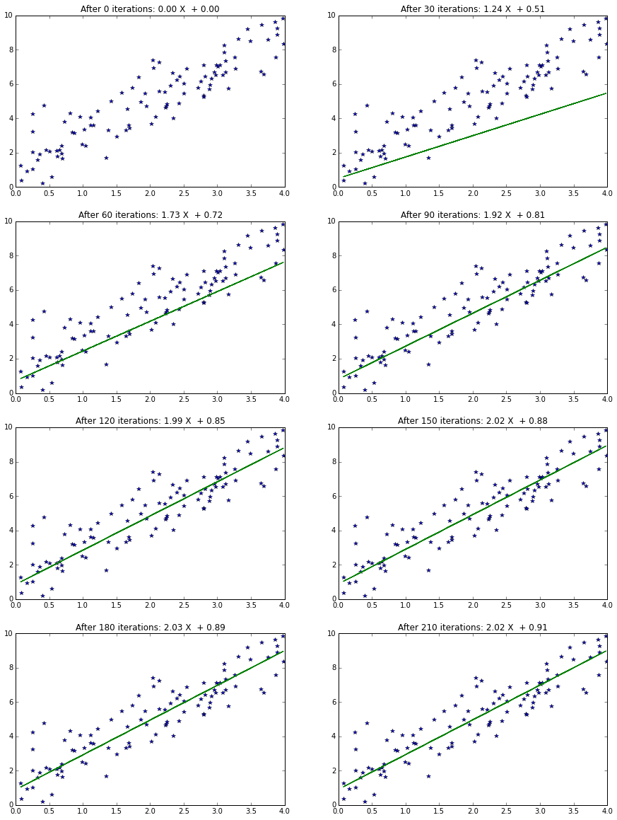
Fig2. RMS error between the line fit and data as training progresses

plt.figure(figsize=(15,20))
for i in np.arange(0,8):
    num_fig = i*30
    Y_pred = W_all[num_fig][0]*X + W_all[num_fig][1]
    plt.subplot(4,2,i+1)
    plt.plot(X,Y,'*',X,Y_pred)
    title_str = 'After %d iterations: %0.2f X  + %0.2f'%(num_fig,
                          W_all[num_fig][0],W_all[num_fig][1])
    plt.title(title_str)

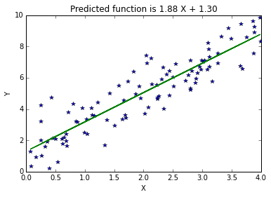
Fig3. Line-fit improves as more iterations are peformed

Line fitting using Pseudoinverse

The same calculations above can be performed using Pseudoinverse.

t0 = time.time()
XTX_inv = np.linalg.inv(np.dot(X_stack.T,X_stack))
XtY = np.dot(X_stack.T,Y)
W = np.dot(XTX_inv, XtY)
Y_pred = W[0]*X + W[1]
tf = time.time()
print 'Pseudoinverse took %0.6f s'%(tf-t0)

title_str = 'Predicted function is %0.2f X + %0.2f'%(W[0],W[1])

plt.plot(X,Y,'*',X,Y_pred)
plt.title(title_str)
plt.xlabel('X')
plt.ylabel('Y')

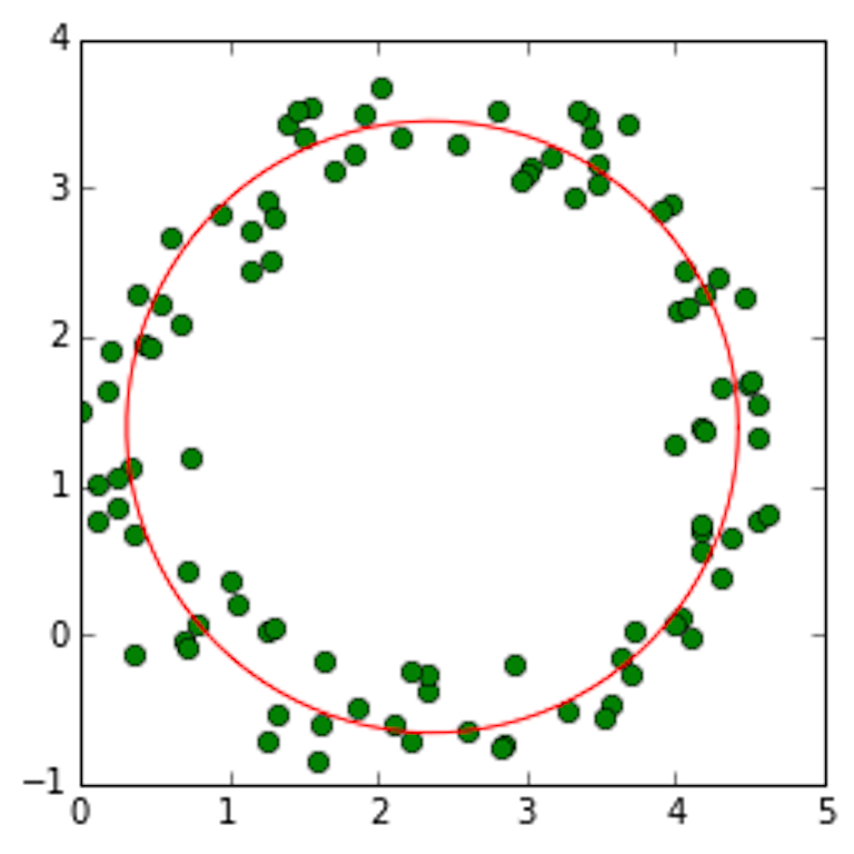
Fig3. Line-fit obtained using pseudoinverse method

Circle fitting

Consider the set of points presented below, where we wish to fit a circle to the curve. Circle is obviosly not a linear function. However, the equation of a circle can be rewritten so the circle equation is linear in terms of unknown parameters, i.e. location of center and the radius. Consider the equation of circle centered at $(x_c,y_c)$ with radius $r$.

$(x - x_c)^2 + (y - y_c)^2 = r^2$

Expanding and regrouping,

$-2x x_c -2 y y_c + \underbrace{x_c^2+y_c^2-r^2}_k = -(x^2+y^2)$ $-2x x_c -2 y y_c + k = -(x^2+y^2)$

The equation above has 3 unknowns, $x_c$,$y_c$ and $k$, and the equation of a circle is linear in these 3 parameters.

Defining $A$ and $b$ as follows $A = \left[ \begin{array}{ccc} \vdots & \vdots & \vdots \\ -2 x & -2 y & 1 \\ \vdots & \vdots & \vdots \end{array} \right]$

$b = \left[ \begin{array}{c} \vdots \\ -(x^2+y^2) \\ \vdots \end{array} \right],$

the circle fitting equation can be written as

$A W = b$

where $ W = [x_c , y_c, k]^T$.

th = np.linspace(0,2*3.14,100)

x = 2.+2*cos(th) + .8*np.random.rand(len(th))
y = 1.+2*sin(th) + .8*np.random.rand(len(th))



A = np.vstack((-2*x,-2*y,np.ones(len(x)))).T
b = -(x**2 + y**2)

ATA_inv = np.linalg.inv(np.dot(A.T,A))
Atb = np.dot(A.T,b)
W = np.dot(ATA_inv, Atb)

x_c = W[0]
y_c = W[1]
r = np.sqrt( x_c**2+y_c**2 - W[2])

x_fit = x_c+r*cos(th) 
y_fit = y_c+r*sin(th) 

plt.figure(figsize=(4,4))
plt.plot(x,y,'go')
plt.plot(x_fit,y_fit,'r')
plt.axis('equal')

print x_c,y_c,r

Fig3. Circle fit obtained by modifying fit function to be linear in parameters

Conclusion

Matrix equations to compute derivatives with respect to a scalar and vector were presented. For cases where the model is linear in terms of the unknown parameters, a pseudoinverse based solution can be obtained for the parameter estimates. These techiques were illustrated by computing representative line and circle fits. In most tasks, pseudo inverse based method is faster, however the describing equation need not be linear in unknown parameters. Pseudoinverse based methods are not suited when working with very large number of parameters, for example linear in parameter neural networks (LPNN).