Linear Algebra review

Vivek Yadav, PhD

This set of notes presents a brief review of Linear Algebra concepts that will be used to develop Control Systems. We will first go over definitions and properties of vector, vector spaces, matrices, etc.

1. Vectors

Vectors are scientific quantities that have both direction and magnitude. Vectors can be as simple as a line segment defined on a 2-D Euclidean plane, or a multi-dimensional collection of numerical quantities. For example, a vector consisting of the position, velocity and acceleration of a given point in the space describes the motion of the particle. Note that the entries in the vector need not be of the same dimension, i.e. a vector can be composed of different quantities. This lets us represent all the variables needed to completely describe a dynamic system using just one vector. A vector is typically denoted by a letter with arrow on top, (for example, $ \overrightarrow {a } $) or a bold lower case letter ($\mathbf{a}$). The later is more common in control systems literature.

2. Vector operations

a) Sum (or difference):

Vector sum (or difference) of two vectors is equal to the vector formed by sum (or difference) of individual elements, and has the same dimension as the original vector. For example, sum of vectors $ \overrightarrow {a} = \left[ 1, 2, 3 \right] $ and $ \overrightarrow {b} = \left[ 3, 3, 4 \right] $ is $\overrightarrow {a}+\overrightarrow {b} = \left[ 1+3, 2+3, 3+4 \right] = \left[ 4, 5, 7 \right].$

and difference is $\overrightarrow {a}-\overrightarrow {b} = \left[ 1-3, 2-3, 3-4 \right] = \left[ -2, -1, -1 \right].$

Vector sum (or difference) is defined only between the vectors of the same dimension.

b) Inner Product:

Inner product of two vectors $\overrightarrow {a} $ and $ \overrightarrow {b}$ is defined as,

$\overrightarrow {a} \circ \overrightarrow {b} = \overrightarrow {a}^T \overrightarrow {b} = \sum_{i=1}^n a_i b_i,$

where $n$ is the length of the vectors $\overrightarrow {a} $ and $ \overrightarrow {b}$.

Inner product, also refered as a dot product has several interpratations.

Inner product represents how similar two vectors are to one another. In the special case where, the vectors are normalized to have unit magnitude, then higher values indicates greater similarity between the vectors. This is also referred as Cosine similarity.
$cos(\theta) = \frac{\overrightarrow {a} \circ \overrightarrow {b}}{ | \overrightarrow {a}| |\overrightarrow {b}|} ,$
Inner product also represents the length of the projection of one vector along the other vector. Therefore, the projection of vector $\overrightarrow {a}$ along vector $\overrightarrow {b}$ is $\frac{\overrightarrow {a} \circ \overrightarrow {b}}{ |\overrightarrow {b}|} .$

c) Outer Product:

Outer product of two vector $ \overrightarrow {a} $ and $ \overrightarrow {b}$ is the matrix $C_{ij}$ such that $C_{ij} = a_i b_j$

Outer product is helpful in certain applications to reduce computation time.

3. Matrices

A matrix (plural matrices) is a rectangular array of numbers, symbols, or expressions, arranged in rows and columns. In control systems, matrices are used to describe how the state vectors (for example position and velocity) evolve and how the control signal influences the state vectors. A matrix is typically denoted by a capital letter ($W$ or $\mathbf{W}$ ). A matrix with $n$ rows and $m\) columns has a dimension of $ n \times m$ matrix and is represented as $A_{n \times m}$ . Further, the $(i,j)$ element of matrix $ A$ is denoted by $a_{i,j}$ .

4. Matrix operations

a) Sum (or difference):

Sum (or difference) of two matrices is equal to the matrix formed by sum (or difference) of individual elements, and has the same dimension as the original matrices. For example, sum of matrices $ A = a_{i,j}$ and $ B = b_{i,j}$ is $C =c_{i,j} = a_{i,j} + b_{i,j} .$

Matrix sum (or difference) is defined between matrices of the same dimension.

b) Product of matrices:

Product of matrix and scalar

Product of a matrix with a scalar is equal to the matrix formed by multiplying each element of the matrix by the scalar. Therefore, $\lambda A = \lambda a_{i,j}$

Product of matrix and matrix

Product of matrices ($AB$) is defined between two matrices $A_{n \times p}$ and $B_{p \times m}$ as,

$C_{n \times m} = A_{n \times p} B_{p \times m} = c_{i,j} = \sum_{k=1}^{p} a_{i,k} b_{k,j},$

where $p$ is the number of columns in $A$ and number of rows in $B$. Note, the matrix product is defined only if the number of columns in $A$ is equal to the number of rows in $B$. The product of the matrices ($C$) is of dimension $ n \times m $. Note, outer product can also be used to compute matrix product, and typically results in lower computation and storage requirements.

$C_{n \times m} = \sum_{k=1}^{p} A_{(i,:)} B_{(:,j)},$

where $A_{(i,:)}$ is the $i^{th}$ row and $B_{(:,j)}$ is the $j^{th}$ column of matrices A and B.

Product of matrix and vector (column space or range)

Product of a matrix with a vector is defined in a similar manner as above, however in the special case of multiplying a matrix by vector results in linear combination of the columns.
$A_{n\times m} b_{m \times 1} = \left[ A_{(:,1)} A_{(:,2)} ... A_{(:,m)} \right] b_{m \times 1}$

Expanding $b_{m \times 1}$ as $[b_1 b_2 … b_m]^T$ and multiplying gives, $A_{n\times m} b_{m \times 1} = b_1 A_{(:,1)}+ b_2 A_{(:,2)}+ ... + b_m A_{(:,m)}$

Therefore, the product of $ A_{n\times m}$ and $b_{m \times 1}$ is a linear combination of the columns of $A$ and the weighing factors are determined by the vector $b_{m \times 1}$. The space spanned by the columns of $A$ is also called the column space or range of the matrix $A$.

Product of vector and matrix (row space)

Product of a vector with a matrix results in linear combination of the rows.
$a_{1\times n} B_{n \times m} = a_{1 \times n} \left[ \begin{array}{c} B_{(1,:)} \\ B_{(2,:)} \\ \vdots \\ B_{(n,:)} \\ \end{array} \right]$

Expanding $a_{1 \times n}$ as $[a_1 a_2 … a_n]$ and multiplying gives,

$a_{1\times n} B_{n \times m} = a_1 B_{(1,:)}+ a_2 B_{(2,:)}+ ... + a_n B_{(n,:)}$

Therefore, the product of $ a_{1\times n}$ and $B_{n \times m}$ is a linear combination of the rows of $B$ and the weighing factors are determined by the vector $a_{1 \times n}$. The space spanned by the rows of $B$ is also called the row space or range of the matrix $B$.

Rank of a matrix

The rank of the matrix is equal to the number of independent rows (or columns). Note, column and row ranks of a matrix are equal. Check the wikipage for a brief description of why.

c) Determinant of a matrices:

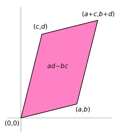
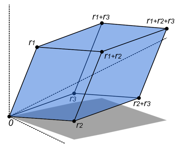
Determinant, defined for square matrices is an estimate of the ‘size’ of a matrix. Determinants represent the volume enclosed by the rows of the matrix in an n-dimensional hyperspace. For a 2-dimensional matrix, the determinant represents area enclosed by the vectors composed of the rows (or columns) of the matrix.

Fig1. Determinant of a 2-dimension matrix is equal to the area of the parallelogram enclosed by the rows (or columns) of the matrix

${\begin{aligned}det(A)={\begin{vmatrix}a&b\\c&d\end{vmatrix}}&=ad-bc.\end{aligned}}$

Fig2. Determinant of a 3-dimension matrix is equal to the volume enclosed by the rows (or columns) of the matrix

${\begin{aligned}det(A)={\begin{vmatrix}a&b&c\\d&e&f\\g&h&i\end{vmatrix}}&=a\,{\begin{vmatrix}e&f\\h&i\end{vmatrix}}-b\,{\begin{vmatrix}d&f\\g&i\end{vmatrix}}+c\,{\begin{vmatrix}d&e\\g&h\end{vmatrix}}\\&=aei+bfg+cdh-ceg-bdi-afh.\end{aligned}}$

Determinant of a full rank square matrix is non-zero, where as the determinant of a rank-deficient matrix is 0.

c) Inverse of matrices:

Inverse of a square matrix is the matrix that when multiplied by the original matrix gives an identity matrix. Identity matrix is a matrix that has 1s for diagonal terms and 0 for all the off-diagonal terms. Inverse of a matrix is computed as the matrix of cofactors divided by the determinant of the matrix, details here. Cofactors of an element $ i,j $ of a matrix is the matrix formed by removing $i^{th} $ column and $j^{th} $ column.

d) Eigen values and eigen vectors:

Consider a vector $\overrightarrow{v}$ such that $A \overrightarrow{v} = \lambda \overrightarrow{v}$ ,

i.e. product of the matrix $A$ times the vector $\overrightarrow{v}$ is the vector $\overrightarrow{v}$ scaled by a factor of $\lambda$. The vector $\overrightarrow{v}$ is called the Eigen vector and the multiplier $\lambda$ is called the eigen value. Eigen values are first computed by solving the characteristic equation of the matrix $det( A - \lambda I) = 0,$

and next the first equation $ A \overrightarrow{v} = \lambda \overrightarrow{v}$ is used to obtain non-trival solution of eigen vectors. Eigen vectors are scaled so their magnitude is equal to 1.

If $V$ is the matrix of all the eigen vectors then, $AV = V \Lambda$ where $\Lambda$ is the matrix whose off-diagonal terms are 0, and diagonal terms are eigen values corresponding to eigen vectors in the columns of $V$. Therefore, $ A = V \Lambda V^{-1}$ or $\Lambda = V^{-1} A V$. In the special case where $V$ is unitary, $ A = V \Lambda V^T$ or $ \Lambda = V^T A V$.

Properties of eigen vectors and eigen values

Eigen vectors are defined only for square matrices. For non-square matrices, singular value decomposition, or SVD is used.
It is possible for a matrix to have repeated eigen values.
Matrix multiplication transforms data in such a way that directions along larger eigen values are magnified.
The space spanned by all the eigen vectors whose eigen values are non-zero is also the column space of the matrix.
If an eigen value is 0, then its corresponding eigen vector is called a null vector. The space spanned by all the null vectors is called the null space of the matrix.
If any of the eigen values is equal to 0, the matrix is not full rank. Infact, the rank of a square matrix is equal to the number of non-zero eigen values.
The determinant of a matrix is equal to product of the eigen values.
Eigen values represent how much the data will get skewed by multiplying it with the matrix A. The eigen vectors corresponding to largest eigen value become dominant while the smaller eigen values’ vectors diminish.

It can be shown that for any integer $n$, $A^n \overrightarrow{v} = \lambda^n \overrightarrow{v}.$ Therefore, if $\lambda<1$, $ A^n \overrightarrow{v}$ goes to zero, and if $\lambda>1$ it goes to infinity. For the special case when $\lambda=1$, $ A^n \overrightarrow{v}= \overrightarrow{v}$. This property is expoited in control system to design control laws that ensure convergence of the system to desired stated by making eigen values less than 1.

Power of a matrix can be computed as $A^n = V \Lambda V^T V \Lambda V^T V \Lambda V^T ... V \Lambda V^T.$ $A^n = V \Lambda (V^T V) \Lambda (V^T V) \Lambda (V^T ... V) \Lambda V^T.$ $A^n = V \Lambda \Lambda \Lambda ... \Lambda V^T.$ $A^n = V \Lambda^n V^T.$

Similarly, exponent of a matrix can be computed as $e^A = V e^\Lambda V^T .$

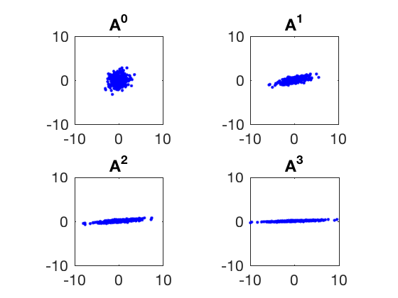
Consider the matrix,

$A = \left[ \begin{array}{cc} 1.5 & 1 \\ 0 & .5 \end{array} \right],$

whose eigen values are 1.5 and 0.5 and eigen vectors are $ [1,0]^T $ and $ [0,1]^T $ respectively. Therefore, multiplying a cloud of randomly dispersed points with $A$ will amplify the components along the first eigen vector and diminish those along the second eigen vector. This is illustrated by the plots below.

clc
close all
clear all

X1 = randn(1,400);
X2 = randn(1,400);

A = [1.2 , 1;
    0 .5];
figure;
for i = 1:4
    Ax = A^(i-1)*[X1 ;X2];
    subplot(2,2,i)
    plot(Ax(1,:),Ax(2,:),'b.')
    axis equal
    axis([-10,10,-10,10])
    title(['A^' num2str(i-1)])
end

Fig3. - Multiplying vectors by a matrix stretches the data along the eigenvector corresponding to the largest eigenvalue.

Properties of eigen values and eigen vectors.

Trace of a matrix (sum of all diagonal elements) is equal to the sum of eigen values
Determinant of a matrix is equal to the product of eigen values.
A set of eigenvectors of $A$, each corresponding to a different eigenvalue of $A$, is a linearly independent set.

Singular value decomposition (SVD)

Singular value decomposition or SVD is a powerful matrix factorization or decomposition technique. In SVD, a $ n \times m$ matrix $A$ is decomposed as $ U \Sigma V^{*} $,

$A = U \Sigma V^*$

where $U$, $ \Sigma $ and $ V $ satisfy

$ U $ is called the matrix of left singular vector, and its columns are eigen vectors of $ A A^{*} $.
$ V $ is called the matrix of right singular vector, and its columns are eigen vectors of $ A^{*} A $.
$ \Sigma $ is a $n \times m $ matrix whose diagonal elements are square root of eigen values of $ A A^{*} $ or $ A^{*} A $.
For most matrices $ n \neq m $, therefore, the maximum rank $A$ can have is the lower of $ m $ or $ n $.
If $ n > m $, then $A $ has more rows than columns and $ \Sigma $ is a matrix of size $ n \times m $ and its $ i,i $ element is square root of eigen value of $ A A^{*} $ or $ A^{*} A $ for $ i = 1$ to $m$.
If $ n < m $, then $A $ has more columns than rows and $ \Sigma $ is a matrix of size $ n \times m $ and its $ i,i $ element is square root of eigen value of $ A A^{*} $ or $ A^{*} A $ for $ i = 1$ to $n$.

Note: $ V^{*} $ is complex conjugate of $V$. If all elements of $V$ are real then $V^{*} = V^T$.

SVD Example:

To better understand SVD, lets apply SVD to a matrix.

$A = \left[ \begin{array}{ccccc} 3 & 4 & 5 & 1 & 2 \\ 1 & 0 & 1.5 & 2 & 1 \\ \end{array} \right]$

SVD in matlab can be computed using ‘svd’ command.

clc
close all
clear all

%% Program to get SVD of a matrix A. 
A = [3,4,5,1,2;
    1,0,1.5,2,1];

[U,S,V] = svd(A)
%% Verify if A = U S V^*
norm_val = norm(A - U*S*V');

fprintf('Difference between A and U S V^* is %0.4f. \n',norm_val)

%% Next lets check if U is eigenvector of A A^* and eigen values are S^2. 
err1 = A*A'  - U*S*S'*U';
fprintf('Difference between A*A^T and U*S*S^T*U^T is %0.4f. \n',norm(err1))
%% Next lets check if U is eigenvector of A^* A
err2 = A'*A  - V*S'*S*V';
fprintf('Difference between A^T*A and V*S^T*S*V^T is %0.4f. \n',norm(err2))

U =

   -0.9617   -0.2741
   -0.2741    0.9617


S =

    7.6897         0         0         0         0
         0    2.0293         0         0         0


V =

   -0.4108    0.0688   -0.6903   -0.4733   -0.3550
   -0.5003   -0.5402   -0.2264    0.6339    0.0693
   -0.6788    0.0356    0.6677   -0.2477   -0.1756
   -0.1963    0.8128   -0.0868    0.5223   -0.1430
   -0.2858    0.2038   -0.1377   -0.1998    0.9044

Difference between A and U S V^* is 0.0000. 
Difference between A*A^T and U*S*S^T*U^T is 0.0000. 
Difference between A^T*A and V*S^T*S*V^T is 0.0000.

Applications of SVD

SVD is a powerful dimensionality reduction technique. Recall, that the eigen vectors of covariance matrix also represent the percentage of explained variance in data. Therefore, square of singular values of a matrix represent the relative amount of data explained by the corresponding eigen vector. In SVD, many singular values are 0, therefore their corresponding vectors do not contribute to the range space of matrix, and can be dropped. This technique results in significant reduction in the number of elements required to describe a matrix, and is typically used as a preprocessing step in dimensionality reduction. This is especially helpful in applications where a storage is an important concern. Truncated or reduced r-dimension approximation is obtained by taking first r-rows of the left and right singular eigenvector matrices and $ r \times r $ submatrix from $S $. Therefore, if we store left and right singular eigenvector matrices, then we need only $r $ numbers to accurately represent the data.

A = [3,4,5,1,2;
    1,0,1.5,2,1];

[U,S,V] = svd(A);

A_reduced = U(:,1:2)*S(1:2,1:2)*V(:,1:2)';
fprintf('Difference between A and reduced representation is %0.4f. \n',norm(A_reduced-A))

Difference between A and reduced representation is 0.0000.

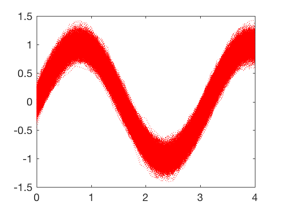
The saving in storage is not clear for the simple example above. Lets consider a little more complex example from signal processing. Say the data from a sensor taken over a duration of 4 seconds as shown in the figure below. To store all the data shown in the figure below, we will need to store $ 41 \times 5000 = 205000 $ values.

clear A

t = 0:.1:4;
for i = 1:5000
    A(i,:) = .1*randn*sin(t) + .1*randn*cos(t) + sin(2*t) + 0.05*randn(1,length(t));
end
figure;
plot(t,A','r:')

Fig4. - Raw signals.

We will apply SVD to obtain a lower dimensional approximation of the signals above. Applying SVD to the matrix, and plotting the explained variance shows that 4 components are sufficient to explain most of the variance in the data.

[U,S,V] = svd(A);
eig_A = diag(S);

for i = 1:length(eig_A)
    epl_var(i) = sum(eig_A(1:i).^2)/sum(eig_A.^2);
end
figure;
plot(epl_var)
axis([1 40 .8 1])

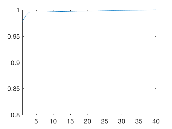
Fig4. - Explained variance vs number of components.

We will therefore, truncate and take only first 4 rows of $ U $ and $ V$, and a $ 4 \times 4 $ submatrix of $ S $. By taking only 4 components, the storage requrirement has reduced from 205,000 numbers to 20,106 $ ( 5000 \times 4+41 \times 4+4 ) $. Therefore, by sacrificing $ 1 \% $ accuracy, we get a 90% saving in storage space. Dimensionality reduction techiques like SVD enable us to convert infinite dimensional system dynamics to finite dimensional differential equations represented in state space form.

A_reduced = U(:,1:4)*S(1:4,1:4)*V(:,1:4)';
figure;
plot(t,A','r:');
hold on ;
plot(t,A_reduced,'k.-');
percent_err = 100.*norm(A-A_reduced)/norm(A);

fprintf('Difference between A and reduced representation is %0.4f %. \n',norm(percent_err))

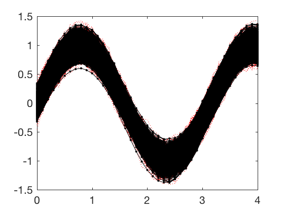
Fig4. Raw signals and signals reconstructed using only.

Difference between A and reduced representation is 1.1752

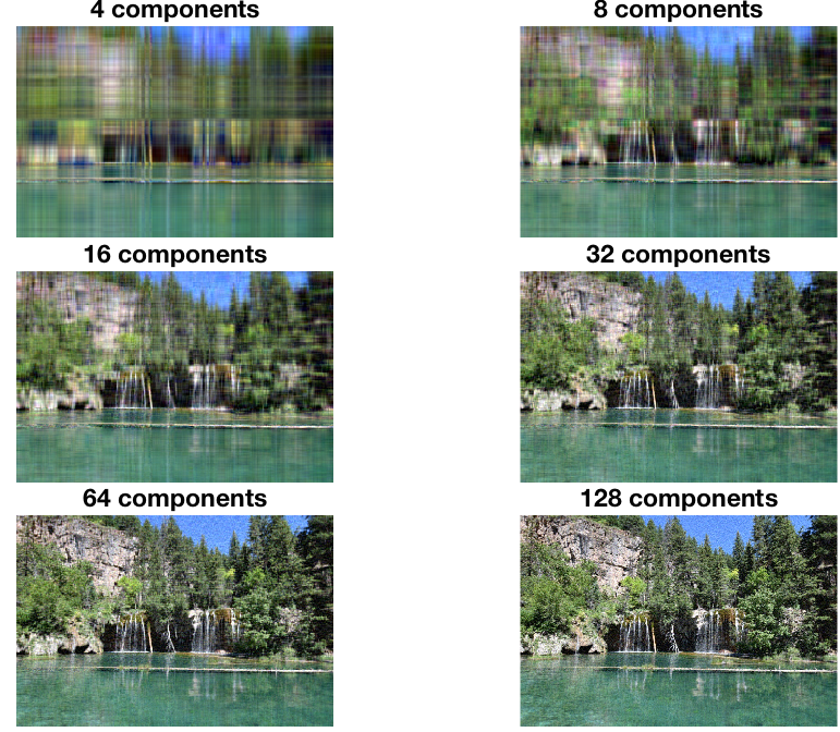
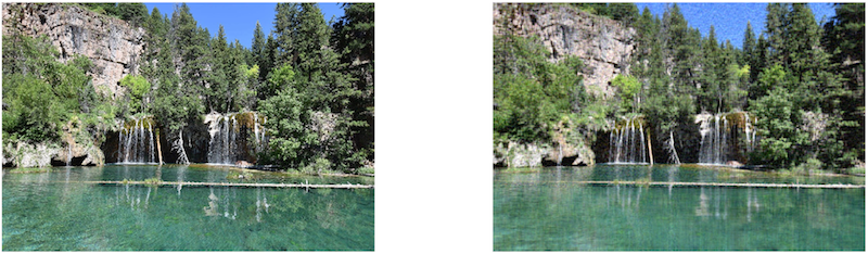
SVD can also be applied to obtain reduced dimension representations of images. Consider the image of Hanging Lake below. Hanging lake is in Colorado, near Glenwood Springs and is famous for its characteristic turquoise color.

A = imread('hanginglake1.jpg');
imshow(A);

Fig5. Beautiful hanging lake near Glenwood Springs, CO.

Images are mathematically represented as a set of 3 matrices each containing intensities of red, blue and green colors. Therefore, we can apply SVD on each matrix of the image, and truncate it differently to test how many components are sufficient to represent the image.

Ar = A(:,:,1);
Ag = A(:,:,2);
Ab = A(:,:,3);
[Ur,Sr,Vr] = svd(double(Ar));
[Ug,Sg,Vg] = svd(double(Ag));
[Ub,Sb,Vb] = svd(double(Ab));

[Ur,Sr,Vr] = svd(double(Ar));
[Ug,Sg,Vg] = svd(double(Ag));
[Ub,Sb,Vb] = svd(double(Ab));

eig_Ar = diag(Sr);
eig_Ag = diag(Sg);
eig_Ab = diag(Sb);

for i = 1:1000
    epl_var(i) = sum(eig_Ar(1:i).^2+eig_Ag(1:i).^2+eig_Ab(1:i).^2);
    epl_var(i) = epl_var(i)/sum(eig_Ar.^2+eig_Ag.^2+eig_Ab.^2);
end

figure;
plot(epl_var)
axis([1 1000 .8 1])

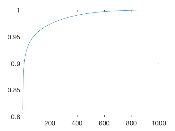
Fig5. Explained variance vs number of components for the image above.

From plot above, we see that more than $ 90 \% $ of covariance is explained by very few components. This is further illustrated below where the reconstructed image is plotted for different number of components. Powers of 2 are selected because many numerical algorithms are faster when dealing with powers of 2 (anecdotal). A good representation of image is obtained for 64 components.

vec_red = [4,8,16,32,64,128];
fig = figure;
p = get(fig,'position');
set(fig, 'position',[0,0,7,5]);
for i=1:length(vec_red)
    ind = vec_red(i);
    Ar_reduced = Ur(:,1:ind)*Sr(1:ind,1:ind)*Vr(:,1:ind)';
    Ag_reduced = Ug(:,1:ind)*Sg(1:ind,1:ind)*Vg(:,1:ind)';
    Ab_reduced = Ub(:,1:ind)*Sb(1:ind,1:ind)*Vb(:,1:ind)';
    A_reduced = A;
    A_reduced(:,:,1)=Ar_reduced;
    A_reduced(:,:,2)=Ag_reduced;
    A_reduced(:,:,3)=Ab_reduced;
    g = subplot(3,2,i);
    imshow(A_reduced);
    p = get(g,'position');
    p(4) = p(4)*1.20; % Add 50 percent to height
    p(3) = p(3)*1.20; % Add 50 percent to width
    set(g, 'position', p);
    title([num2str(vec_red(i)) ' components']);    
end

Fig6. Reconstructed images for different number of components.

ind = 64;


Ar_reduced = Ur(:,1:ind)*Sr(1:ind,1:ind)*Vr(:,1:ind)';
Ag_reduced = Ug(:,1:ind)*Sg(1:ind,1:ind)*Vg(:,1:ind)';
Ab_reduced = Ub(:,1:ind)*Sb(1:ind,1:ind)*Vb(:,1:ind)';
A_reduced = A;
A_reduced(:,:,1)=Ar_reduced;
A_reduced(:,:,2)=Ag_reduced;
A_reduced(:,:,3)=Ab_reduced;


fig = figure;
p = get(fig,'position');
set(fig, 'position',[0,0,12,4]);
subplot(1,2,1);
imshow(A);
subplot(1,2,2);
imshow(A_reduced);

err_r = norm(double(Ar) - Ar_reduced)/norm(double(Ar));
err_g = norm(double(Ag) - Ag_reduced)/norm(double(Ag));
err_b = norm(double(Ab) - Ab_reduced)/norm(double(Ab));
err_avg = (err_r+err_g+err_b)/3*100;

fprintf('Difference between original and reduced image is %0.4f %. \n',err_avg);

Fig7. Original image and image reconstructed with 64 components.

Difference between original and reduced image is 2.2255

By choosing 64 components a $ 1000 \times 1500 \times 3 $ or 4.5 million element matrix is reduced to $ (1000 +1500+1) \times 64 \times 3 $ or 480192 element matrix, about 90% saving in storage at the cost of 2% accuracy.

Systems of equation

In control theory, we often come across equations of the form $ A_{n \times m} x_{m \times 1} = b_{n \times 1} $ where given $A$ and $b$, we wish to solve for $x$. Lets consider the following cases,

When $n = m $, in this case the matrix $A$ is a square matrix and a unique solution $ x = A^{-1} b $ exists if $ A$ is full rank. If $A$ is not full rank, then no solutions exist if $b$ has a component along the null space of $A$.
When $n > m $, in this case, there are more equations (or constraints) than free parameters. Therefore, it is not possible to find a solution that solves $ A x = b$ for any $ x $. Such equations typically arise when we want to estimate some parameter from multiple observations. A typical approcah to solve such type of equations is to formulate an error function (sum of squared errors), and find parameters that minimize it.
When $m > n $, in this case, there are more unknowns than equations, and solution exists if rank of $A$ is equal to $n$. If $A$ is not full rank, then $Ax$ cannot have components along null space of $A$. Therefore, if $b$ has a component along null space of $A$ then solutions do not exist. These types of equations are very common in control synthesis, where there are multiple ways to control the same system to achieve the same goal. Typically controller parameters are varied to minimize certain cost that combines task and control effort.

Cayley-Hamilton Theorem

Cayley-Hamilton Theorem states that a matrix satisfies its own equation. Recall, characteristic equation of $A$ is,

$det( A - \lambda I) = 0,$

Substituting $A$ in place for $ \lambda $ gives, $det( A - A I)=det( A - A )= det( 0) = 0,$

$C(\lambda) =det( A - \lambda I) = \lambda^n + \alpha_1 \lambda^{n-1}+ \alpha_2 \lambda^{n-2}+ \dots + \alpha_0 = 0 ,$

where $C$ is characteristic polynomial. We also have

$C(A) = A^n + \alpha_1 A^{n-1}+ \alpha_2 A^{n-2}+ \dots + \alpha_0 I = 0.$

Cayley-Hamilton theorem can be applied to calculate analytic functions of matrix. It is in particular useful to compute exponetials of matices. First consider a polynomial function $P(s)$ whose order is greater than $n$. We can write $P(A)$ as,

$P(A) = Q(A) C(A) + R(A),$

where $Q$ is analogous to quotient and $R$ is analogous to remainder when the polynomial $ P(s) $ is divided by the characteristic polynomial. Note $R$ is a polynomial or order less than $n$. As $C(A)=0$, we have

$P(A) = R(A).$

Note, as eigen values also satisfy the characteristic equation, we also have $ P(\lambda_i) = R(\lambda_i) $ for each $ \lambda $.

The process to compute $ P(A) $ is as follows,

Express $R(s)$ as $ a_0 + a_1 s + a_2 s^2 + \dots + a_{n-1} s^{n-1} $
Use $ P(\lambda_i) =R(\lambda_i) $ to obtain $n-1$ equations.
Express $ n-1 $ $ P(\lambda_i) =R(\lambda_i) $ as a system of equations in unknowns $a_0$ to $a_{n-1}$
Solve for the unknowns using gaussian elimination or inverting the matrix.

The same process can be applied to compute any analytical function of a matrix. This process is illustrated by an example below.

Example:

Given

$A = \left[ \begin{array}{cc} 0 & 1 \\ -2 & -3 \end{array} \right],$

calculate $ e^{A t}$

Solution

Characteristic equation of $A$ is given by

$0 = det \left( \left[ \begin{array}{cc} 0 & 1 \\ -2 & -3 \end{array} \right] - s \left[ \begin{array}{cc} 1 & 0 \\ 0 & 1 \end{array} \right] \right),$ $0 = det \left( \left[ \begin{array}{cc} -s & 1 \\ -2 & 3-s \end{array} \right] \right) = s^2 + 3 s + 2$

Therefore, eigen values of $A$ are -2 and -1.

Using Cayley-Hamilton theorem,

$e^{A t} = a_0 I + a_1 A$

As eigen values also satisfy the characteristic equation, we have

$e^{-t} = a_0 - a_1$ $e^{-2t} = a_0 - 2 a_1$

Solving for $ a_0 $ and $ a_1 $ gives,

$a_0 = 2 e^{-t} - e^{-2t}$ $a_1 = e^{-t} - e^{-2t}$

Therefore, exponential of $ e^{At} $ is

$e^{A t} = (2e^{-t} - e^{-2t}) I + (e^{-t} - e^{-2t}) A$

Cayley-Hamilton theorm is very powerful and is used extensively to analyze dynamic systems. As we will see in coming classes, it is used to derive rules to test if a dynamic system is controllable, if the states can be observed given measurement and the system, etc.