System dynamics and State-space Representations

System dynamics is a mathematical approach to understanding the behavior of complex systems over time. System dynamics allow a control designer to predict how the plant or a system responds to actuator commands and external disturbances. System dynamics are used to design optimal control signals and observers to estimate variables that define the current state of the system. Figure below shows how system dynamics model fit into design of control systems.

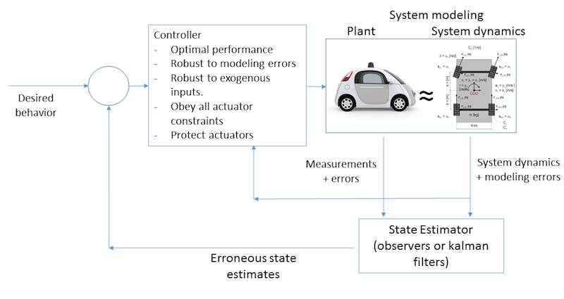
Fig 1. - Overview of a typical control system

For the example above, the system dynamics model is used to obtain estimates of position and heading of the car from sensor measurement. These estimates are then fed into the controller which utilizes the system dynamics model along with estimates of position and velocity to generate a control law to be applied to the car’s actuators. In summary, system dynamics model is used convert measurements to estimates of the values necessary to describe what the system is doing, and for designing the control law.

System dynamics modeling considerations

“All models are wrong, some are useful” ~ George Box.

The quote above accurately characterizes the nature of models. In real-world applications, it is not possible nor is necessary to design a detailed model of the system that we wish to control. The system modeling process often involves several simplifying assumptions, and the level of detail to consider or exclude is a decision that one will have to make as a control designer.

How much detail is enough for modeling?

Consider the example of a car of mass $m $ moving along a straight line under the influence of a force $ F $. The acceleration of the particle along the line that is parametarized by $x $ is given by,

$\ddot{x} = \frac{F}{m}$

The equation above is a sufficient model of the car if we are interested only in its rectilinear motion. However, it is not a good representation of how a car behaves in the real world, where motion is in a plane, and directions cannot be changed instantaneously. A slightly more complex model of the car is refered to as the unicycle model, whose equations of motion are given by,

$\dot{v} = \frac{F}{m},$ $\ddot{\theta} = \frac{\tau}{I}$

with the kinematic constraints,

$\dot{x} = v cos(\theta)$ $\dot{y} = v sin(\theta)$

where $x $ and $y$ define the position of the car, and $\theta $ defines the orientation. $ \tau $ is the turning torque input and $ I $ is the moment of inertia. This model is a little more informative than the particle mass moving along a straight line, as it captures the turning dynamics of the car. However, it is not complete, as it does not capture the fact that the car cannot change its direction instantaneously. Including this aspect in the model results in bicycle model of a car. This model captures both the turning and rectilinear dynamics of a car. However, such a model is not complete, because it ignores, suspension dynamics, friction, effect of drag, delay due to actuator response, etc. A more complex representation of the car can be formulated that includes mathematical models of all these phenomena, however, the choice of weather to include or not is a judgement call that a control designer makes. A very complex model results in a model with several parameters that need to be estimated, and any error in estimation of them can result in erroneous control. On the other hand, an over-simplistic system model can result in generation of control commands that are not realizable by the car, and in some cases can cause damage to the car itself.

Using different system dynamics model for different tasks of the controller.

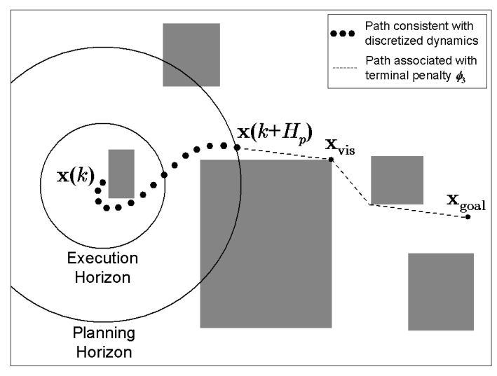
In many applications, it is not efficient to use a detailed model of the system. A detailed model is useful for generating control signals that do not violate the dynamics of the system. For example, a detailed model of a car is needed to avoid situations where the heading of car is commanded to change without changing position along its length. However, a detailed model is not as important for applications where we are interested in a gross performance measure, such as minimum-time trajectory between two points on a map. In this case, using a detailed model of the car will further complicate the already complex task of finding the shortest path between two points. In such cases, a point mass model is used to compute the fastest path, and a detailed model is used to generate commands to follow that path. This process of separating the control task into multiple levels is also referred as a hierarchical control scheme. Below is one such example where an obstacle-free trajectory is first obtained by completely ignoring the dynamics, next a discretized UAV model with actuator contrainsts is used to generate smoother trajectory, and finally the actual UAVs model is used to generate commands for its actuators.

Fig 2. - Receding horizon control example

Types of system dynamics models: Continuous, discrete and hybrid

System dynamic models are typically represented using either differential equations or difference equations, and in some special cases both. Differential equations relate variables of interest to their derivatives, and the difference equations recursively define the next values of a set of variables given their current values. This leads to 3 types of system dynamic models,

Continuous models: Continuous system dynamic models are models that are continuous in time. Such models are described using differential equations. For example, equations of motion of car moving on a 2-D surface, an object falling under the effect of gravity, etc.
Discrete models: Discrete system dynamic models are models that are discrete in time, where states are defined after a fixed interval of time. Such models are described using difference equations. All differential equations can be expressed as a difference equation by using appropriate discretization (but not vice versa). In addition, examples of systems that can be modeled as discrete models are, closing price of a stock index, macroeconomic descriptors of economy, etc.
Hybrid models: In some cases, it is not possible to describe the system using either continuous or discrete models, and both are required to capture what the system is doing. Such models are called hybrid system models. For example, models of humanoid walking involves two phases, a single stance phase where one leg is on ground and other in the air, and a double stance phase where both legs are on the ground. Describing such dynamics requires modeling both the single and double stance phases, and discrete conditions when the switch from single to double stance phase occurs. Another example is of viral dynamics where the concentration of virus in the body is described using continuous equations, and the delivery of the drug is modeled as a discrete event.

** Note: Although most systems are nonlinear, in many instances the system dynamics model can be approximated by a linear model, and this approximation is often sufficient for generating sub-optimal control commands. Further, linear systems allow us to develop computational tools for understanding the behavior of a systems and devloping control laws that are applicable to all linear systems. This understanding can be extended to study and design controllers for more complex nonlinear systems. We will therefore, study linear systems first, and work with nonlinear systems later in the course. An example of linearization applied to nonlinear system can be found here. **

State space representations:

There are many ways to represent the same system dynamics. State space approach is perhaps the most commonly used method to model the dynamics of a system. State-space representation is a mathematical model of a physical system as a set of input, output and state variables related by first-order differential (or difference) equations. ‘State space’ refers to the multi-dimensional space spanned by the state variables. The state of the system can be represented as a vector within this space. To understand this definition further, lets look at the individual terms in this definition.

1. State variables

The state variables are a set of system variables that can completely describe the system at any given time. If the state variables are chosen such that they represent a smallest possible number of variables requires to completely describe the system, then the number of state variables is equal to the order of the system.

2. Input variables

Input variables refer to the control signals or user applied inputs to the system.

3. Output variables

In most cases, the states of a system are monitored using measurements from the sensors of a system. These measurements need not directly provide any information about the state of the system. In such cases, its the task of the control system designer to design obervers or estimators to convert sensor measurements into state estimates that can be used by the controller.

4. First-order differential (or difference) equations

First order differential equations relate variables to their first order derivatives, and first order difference equations relate values at current time-step to the next. All systems represented in a state-space form have to be comprised of first order differential (or difference) equation.

If the states satisfy an additional contraint that given the current state of the system, the future states of the system are completely determined by the current state and applied control input. The system dynamics described in this way is memoryless, i.e. the future states do not depend on the past state history or how the current state was achieved. Such processes are also refered as Markov processes (for continuous time) or Markov chains (for discrete time). In cases where the system dynamics is of second order, we split the second order equations into two first order equations.

State space representations: Nonlinear systems

In general, state space representation for a continuous nonlinear system is given by

$\dot{x} = f(x,u),$

and

$y = h(x,u),$

where $ x $ is a vector of state variables, $ u $ is a vector of input variables, and $ y $ is a vector of output variables. The vectors functions $ f $ and $ h $ represent the system dynamics and measurement respectively. In the special case where the system dynamics can be expressed as

$\dot{x} = f(x) + g(x) u,$

the system is called control-affine.

Similarly, state space representation for a discrete nonlinear system is given by

$x[k+1] = f(x[k],u[k]),$

and

$y[k] = h(x[k],u[k]).$

A control affine discrete system can be represented as, $x[k+1] = f(x[k]) + g(x[k]) u[k]$

State space representations: Linear systems

In the special case where the system is linear in state, input (or control) and output variables, the system dynamics can be represented using matrices.

Continuous time linear system dynamics model:

Continuous time linear system dynamics are modeled as,

$\dot{x} = A(t) x(t) + B(t) u(t),$

where $ A(t) $ is called the system matrix and $ B(t) $ is called the input matrix. Measurements in this case are given by

$y(t) = C(t) x(t) + D(t) u(t) ,$

and $ C(t) $ is the output matrix and $ D(t) $ is the feedforward matrix.

In special case where the matrices $ A, B, C $ and $ D $ are all time-invariant, the system is called linear time-invariant (or LTI) system, and can be described as,

$\dot{x} = A x(t) + B u(t),$ $y(t) = C x(t) + D u(t) .$

Discrete linear system dynamics model:

Discrete linear system dynamics are modeled as,

$x[k+1] = A[k] x[k] + B[k] u[k],$

where $ A[k] $ is the system matrix and $ B[k] $ the input matrix. Measurements are given by

$y[k] = C[k] x[k] + D[k] u[k] ,$

and $ C[k] $ is the output matrix and $ D[k] $ is the feedforward matrix.

As before, a discrete linear time-invariant discrete system is represented as

$x[k+1] = A x[k] + B u[k],$ $y[k] = C x[k] + D u[k] .$

State-space representation: Example

Consider the example of the particle mass,

$\ddot{x} = \frac{F}{m}$

This is a second order system in the position $ x$. To make it a first order system, we define two variables, position and velocity as follows,

$x_1 = x$ $x_2 = \dot{x}_1 = v$

The original system dynamics equation can now be written as,

$\dot{x}_2 = \frac{F}{m} .$

The state space variables now are $ x_1 $ and $ x_2 $, and the state-space representation is

$\underbrace{\frac{d}{dt} \left[ \begin{array}{c} x_1 \\ x_2 \end{array} \right]}_{\dot{X}} = \underbrace{\left[ \begin{array}{cc} 0 & 1 \\ 0 & 0 \end{array} \right]}_A \underbrace{\left[ \begin{array}{c} x_1 \\ x_2 \end{array} \right]}_X + \underbrace{\left[ \begin{array}{c} 0 \\ \frac{1}{m} \end{array} \right]}_B \underbrace{F}_u$

Say the measurements we have in this case are the positon $ (x) $ and the force $ (F) $, the measurement equations can be written as,

$y = \underbrace{\left[ \begin{array}{cc} 1 & 0 \\ 0 & 0 \end{array} \right]}_C \underbrace{\left[ \begin{array}{c} x_1 \\ x_2 \end{array} \right]}_X + \underbrace{\left[ \begin{array}{c} 0 \\ 1 \end{array} \right]}_D \underbrace{F}_u$

State-space representation: Discretization

Discretization refers to transforming a continuous processes into a discrete process by approximating the variables of the continuous system with a smaller sample, typically taken at fixed intervals along time-axis. As we will see later in the course, optimal control laws or minimum cost trajectories/paths are required to minimize a given cost function while statisfying the system dynamic equations each point in time. As time is a continuous variable, this results in an infinite dimensional problem, which can be computationally intractable. Approximating a continuous system with discrete system significantly reduces the complexity of the solution process. Consider the continuous-time dynamic system given by

$\dot{x} = A x(t) + B u(t),$ $y(t) = C x(t) + D u(t) .$

The derivative can be approximated using euler’s difference formula as,

$\dot{x} \approx \frac{x(t+\Delta t) - x(t) }{ \Delta t} ,$

and by sampling at fixed intervals, time can be reindexed by an iterator $ k $. The derivative now becomes

$\dot{x} \approx \frac{x[k+1] - x[k] }{ \Delta t} .$

The system dynamics equations can therefore be written as

$\frac{x[k+1] - x[k] }{ \Delta t} \approx A x[k] + B u[k].$

Rearranging the terms gives,

$x[k+1] \approx \underbrace{(I + A \Delta t)}_{A_d} x[k] + \underbrace{B \Delta t}_{B_d} u[k].$

** Note: Choice of $ \Delta t $ is very crucial in discretizing a continuous time system. Choosing a very small $ \Delta t $ results in an approximation with large number of contraint equations, and a very large $ \Delta t $ can result in large approximation error. These errors are also referred to as discretization errors. **

State-space representation: Applications

Almost all real-world phenomena can be represented using state-space methods. Applications range from predicting regions in brain that are involved in mental processes, developing optimal drug delivary schemes to minimize viral load, parameter estimation for machine learning/artificial intelligence algorithms, and control of self-driven cars and robots. Below are some examples,