Direct collocation for optimal control

Vivek Yadav

In the previous class, we derived conditions of optimality and saw how the Riccati equation can be solved to compute optimal control. We next looked into a family of direct optimization methods called shooting methods. We derived optimal control using single shooting. In single shooting, first a control scheme is chosen, then the states are integrated forward in time, and the optimizer tries to find control that minimizes some cost under equality constraints imposed at the end of the interval. In single shooting, the constraint, depends on the control applied until that point, further any change in the control policy will affect the final error. Further, as we are integrating over entire time-domain, errors will accumulate, and the defect at the end depends on the entire control policy. A big drawback of single shooting method is that there is no guarantee that the intermediate controllers that an optimizer iterates over lead to stable performance, and it is possible that for some choice of control, the states go to infinity. Multiple shooting alleviates some of these issues. In multiple shooting, we discretize the control policy as a piecewise linear (or constant) control policy, and descretize states at these points. We integrate from start of the interval to the end, and enforce the condition that the states at the end of the interval are the initial value for the next interval. This method results in good convergence because the effect of changing control input at each discretization step is captured by one defect. However, the optimization process is slow, because we numerically integrate the states from the start of the interval to the end. Direct collocation methods are a set of methods developed to address these specific concerns.

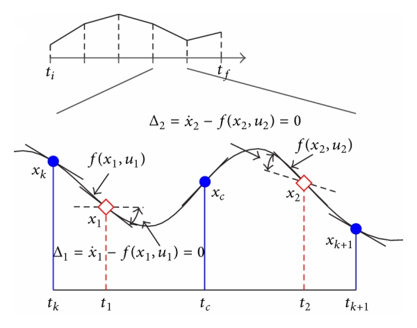
Direct collocation is a very powerful nonlinear optimization technique in which we approximate state and control using piecewise continuous polynomials, and exploit properties of these polynomials to simplify the involved integration calculations. As integration and other involved calculations are converted to algebraic equations, the time to compute these parameters significantly decreases. In direct collocation, the constraints on dynamics are imposed on intermediate points (called collocation points). The optimial solution is required to satisfy the conditions of optimality at these intermediate points only. This idea of direct collocation is expressed in the figure below,

Fig 1. Main idea of direct collocation: To minimize the error between state derivatives from dynamics and from polynomial differentiations.

Taken from Survey of direct transcription for low-thrust space trajectory optimization with applications

A simple direct collocation algorithm can be implemented as follows. After approximating control by piecewise continuous linear function, we next approximate states by piecewise continuous cubics such that the value at each knot (discretization) points is equal to state value, and derivative is equal to derivative from system dynamics. Note, once the states and derivatives at the knot points are fixed, the cubic between the knot points is completely defined. Therefore, the intermediate values can only be changed by changing the state or derivative (via control). Now enforce the condition that the derivative of the piecewise continuous cubic must be equal to the state derivative computed from system dynamics condition. A good review of direct collocation techniques can be found here. Sometimes discrete variable methos are also called pseudo-spectral methods. Direct collocation scales well to complex problems, and has been applied to problems such as, designing gaits for humanoid walking, satellite trajectory planning, obstacle free trajectory planning for robots, path planning of unmanned aerial vehicles (UAVs or drones). Below are a few examples of direct collocation in action,

1. Direct collocation: Algorithm

Direct collocation involves 3 main components that define the type of direct collocation method,

Choice of piece-wise polynomial to represent state and control: For states, piecewise cubic polynomials are a good choice. However, depending on the specific problem domain, some methods may be preferred over another. For example, in trajectory optimization of walking robots, Bezier polynomials, in other application Legendre polynomials may be preferable.
Method of integrating cost function: Cost function is typically chosen as an integral term that depends on the entire trajectory. The integration process can be converted to summation using a fewer intermediate values. The method of numerical integration is also called quadrature.
Method of state-propogation between time points: In addition to integrating the total cost, we need to integrate from the start of interval to some other point.

Direct collocation methods are named based on the choice of polynomials to represent the state variables, the method of numerical integration (quadrature) of cost function, and state-propogation scheme used to dervive the corresponding nonlinear programming method. If the step 3 is used, then the collocation is called integral collocation method. In cases where, the integration in step 3 is not performed, and the derivative is estimated at midpoint using the state and dynamics values at knot points, the technique is called differential collocation method. Midpoint is chosen because for a cubic with fixed end points (value and derivative), the derivative at the midpoint is farthest away from either of the derivatives. Note, for a cubic polynomial, once the derivatives and state values are defined at the interval, the cubic is completely defined in the corresponding interval, values at midpoint can be changed only by changing the state values and their derivatives. We will work out a specific direct collocation method called the Hermite-Simpson collocation method to better understand the process.

2. Problem formulation,

The control problem that we are trying to solve, can be expressed as: Find a control sequence to minimize,

$J(u) = \Phi(X_f) + \int_{t=0}^{t_f} L(t,X,u) dt .$

Subject to,

$\dot{X} =f(x,u),$

with initial condition $ X(0) = X_0 $, under constraints,

$u_{min} \leq u \leq u_{max},$ $X_{min} \leq X \leq X_{max},$ $C_{eq}(X,u) = 0 ,$ $C(X,u) \leq 0 ,$

3. Hermite-Simpson collocation method

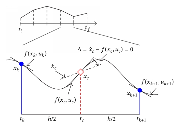
In Hermite-Simpson collocation method, the state trajectories are expressed as cubic polynomials, and the control is expressed as a piecewise linear function. The dynamic equations are imposed as constraints at collocation points that are midpoints of the discretization intervals. The Hermite-Simpson collocation method can be implemented as follows,

1. Discretize:

Say we discretize time $ t_f $ into $ N $ intervals as,

$t_0 = 0 \leq t_1 \leq t_2 \leq \dots \leq t_{k} \leq t_{k+1} \dots \leq t_{N}=t_f$

The states between $ t_k $ and $ t_{k+1} $ can be written as,

$X(t) = a_{k,0} + a_{k,1} t + a_{k,2} t^2 + a_{k,3} t^3 ,$

which gives

$\dot{X}(t) = a_{k,1} + 2 a_{k,2} t + 3 a_{k,3} t^2 ,$

where $ a_{k,0} $, $ a_{k,1} $, $ a_{k,2} $ and $ a_{k,3} $ are coefficients of the polynomial approximation in $ k^{th} $ interval.

2. Compute state derivatives at the collocation point:

Collocation point is the midpoint of the interval

$t_{k,c} = \frac{t_k+t_{k+1}}{2}$

As the value of the state or its derivatives will not change by shifting the interval from $ [t_k,t_{k+1} ] $ to $ [0,h ] $, where $ h = t_{k+1} - t_k $, we shift the time interval. We now have,

$X(0) = X_k$ $X(h) = X_{k+1}$ $\dot{X}(0) = \dot{X}_{k} = f(X_k,u_k )$ $\dot{X}(h) = \dot{X}_{k+1} =f(X_{k+1},u_{k+1} )$

The same can be computed from the polynomial representations too. This gives us,

$\left[ \begin{array}{c} X(0) \\ \dot{X}(0) \\ X(h) \\ \dot{X}(h) \end{array} \right] = \left[ \begin{array}{cccc} 1 & 0 & 0 & 0 \\ 0 & 1 & 0 & 0 \\ 1 & h & h^2 & h^3 \\ 0 & 1 & 2 h & 3 h^2 \end{array} \right] \left[ \begin{array}{c} a_{k,0} \\ a_{k,1} \\ a_{k,2} \\ a_{k,3} \end{array} \right]$

Taking the inverse gives,

$\left[ \begin{array}{c} a_{k,0} \\ a_{k,1} \\ a_{k,2} \\ a_{k,3} \end{array} \right] = \left[ \begin{array}{cccc} 1 & 0 & 0 & 0 \\ 0 & 1 & 0 & 0 \\ -\frac{3}{h^2} & -\frac{2}{h} & \frac{3}{h^2} & -\frac{1}{h} \\ \frac{2}{h^3} & \frac{1}{h^2} & -\frac{2}{h^3} & \frac{1}{h^2} \end{array} \right] \left[ \begin{array}{c} X(0) \\ \dot{X}(0) \\ X(h) \\ \dot{X}(h) \end{array} \right]$

With these coefficients, we can compute the value of states and their derivatives at collocation points as,

$X_c = X \left( \frac{h}{2} \right) = \frac{1}{2} \left( X_k + X_{k+1} \right) + \frac{h}{8} \left[ f(X_k,u_k) - f(X_{k+1},u_{k+1}) \right]$

The time-derivative at midpoint is given by,

$\dot{X}_c = \dot{X} \left( \frac{h}{2} \right) = - \frac{3}{2 h} \left( X_k - X_{k+1} \right) - \frac{1}{4} \left[ f(X_k,u_k) + f(X_{k+1},u_{k+1}) \right]$

This derivative depends on the states and control at the interval or knot points. By choosing the states and controls appropriately, we can make sure that the derivative at the collocation point matches the dynamics. The control at the collocation point is given by

$u_c = \frac{u_k+u_{k+1}}{2}$

We construct a defect $ \Delta_k $ for each interval such that,

$\Delta_k = \dot{X}_c - f(X_c, u_c)$ $\Delta_k = - \frac{3}{2 h} \left( X_k - X_{k+1} \right) - \frac{1}{4} \left[ f(X_k,u_k) + f(X_{k+1},u_{k+1}) \right] - f(X_c, u_c)$ $\Delta_k = - \frac{3}{2 h} \left[ \left( X_k - X_{k+1} \right) + \frac{h}{6} \left[ f(X_k,u_k) + 4 f(X_c, u_c)+ f(X_{k+1},u_{k+1}) \right] \right]$

We redefine the state constraint as,

$\Delta_k = \left[ \left( X_k - X_{k+1} \right) + \frac{h}{6} \left[ f(X_k,u_k) + 4 f(X_c, u_c)+ f(X_{k+1},u_{k+1}) \right] \right]$

The last term in the expression above is implicit Hermite integration of system dynamics. We call this integration implicit because the last term in the bracket is equal to the Hermite integration only when the collocation point satisfies the system dynamics.

3. Express cost-function in terms of optimization parameters.

The next step is to approximate the cost function, we can compute the cost function using various numerical integration (or quadrature) schemes. Say we choose to use trapezoid method, the cost function expressed as,

$J(u) = \Phi(X_f) + \int_{t=0}^{t_f} L(t,X,u) dt .$

We can use trapezoid integration and integrate the above in an interval as

$J_{nlp} = \Phi(X_{N}) + \frac{1}{2}\sum_{k=1}^{N-1} \left( L(t_{k+1},X_{k+1},u_{k+1}) + L(t_k,X_k,u_k) \right)(t_{k+1}-t_k) .$

For the special case where we have linear quadratic regulator, with time points discretized evenly at intervals of $ h $, we have

$J_{nlp} = \Phi(X_{N}) + \frac{1}{2}\sum_{k=1}^{N-1} \left( X_{k+1}^T Q X_{k+1} + u_{k+1}^T R u_{k+1} +X_{k}^T Q X_{k} + u_{k}^T R u_{k} \right) h.$

4. Define additional constraints

The constraints on states and controls can be expressed as

$u_{min} \leq u_k \leq u_{max},$ $X_{min} \leq X_k \leq X_{max},$ $C{eq}(X_k,u_k) = 0 ,$ $C(X_k,u_k)\leq 0 ,$

4. Problem formulation: Nonlinear programming

Using items 1 through 4, the optimal control can be rewritten as,

$\underbrace{minimize}_{X_k,u_k} \left( \Phi(X_{N}) + \frac{1}{2}\sum_{k=1}^{N-1} \left( X_{k+1}^T Q X_{k+1} + u_{k+1}^T R u_{k+1} +X_{k}^T Q X_{k} + u_{k}^T R u_{K+1} \right) h. \right)$

Subject to,

$\Delta_k = \left[ \left( X_k - X_{k+1} \right) + \frac{h}{6} \left[ f(X_k,u_k) + 4 f(X_c, u_c)+ f(X_{k+1},u_{k+1}) \right] \right] = 0$ $u_{min} \leq u_k \leq u_{max},$ $X_{min} \leq X_k \leq X_{max},$ $C{eq}(X_k,u_k) = 0 ,$ $C(X_k,u_k)\leq 0.$

** Note, in the formulation above, we need not compute any integrals, and all the functions are simple algebraic operations (additions and multiplications). Further, as all the functions are algebraic functions, it is very easy to compute the derivative of the functions. Providing derivative information significantly improves convergence properties of the nonlinear program solvers. Regardless, the direct collocation gives convergent solutions that approximate the optimal control well. It can be shown that for sufficiently small interval, the error between the optimal control and controller generated by using direct collocation can be made smaller than any desired threshold. **

** The complete name of the nonlinear programming problem above is cubic Hermite-Simpson derivative collocation with trapezoid quadrature. **

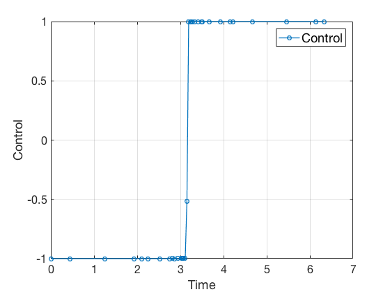
Bang-bang control

Lets consider the a example of designing control for a double integrator whose control can vary between -1 and 1. If we want to reach from some starting point say 0 to 10, the fastest control solution is to apply 1 control for half the time, and then apply -1, i.e. accelerate as fast as possible, and at the right time swithc from acceleration to deceleration to slow down as fast as possible. Lets see how well this control strategy is approximated by the direct collocation method (cubic Hermite-Simpson derivative collocation with trapezoid quadrature method).

Problem formulation,

Given the double integrator system $ \ddot{X} = u $,

$minimize (t_f)$

given,

$-1 \leq u \leq 1$ $X_0 = 0, X_f = 10.$

Solution

We describe control as a piece-wise constant function, and the position and velocity variables defined at the knot points form the additional input to the optimizer. We then integrate the states starting with one knot point to another assuming this control and apply equality constraints between this and the next point. The code snippet below shows this. Complete MATLAB code different examples can be found here.

%% Constraint function

function [C,Ceq]=cons_fn(X_opt)

N = (length(X_opt)-1)/3;
N_st = 2; 
t_f = X_opt(1);
x = X_opt(N+2:end);
u = X_opt(2:N+1);
x = reshape(x,N,N_st);
t = linspace(0,1,N)'*t_f;
dt = t(2) - t(1);

tc = linspace (t(1)+dt/2,t(end)-dt/2,N-1);

xdot = innerFunc(t,x,u);
xll = x(1:end-1,:);
xrr = x(2:end,:);
xdotll = xdot(1:end-1,:);
xdotrr = xdot(2:end,:);
ull = u(1:end-1,:);
urr = u(2:end,:);

xc = .5*(xll+xrr)+ dt/8*(xdotll-xdotrr);
uc = (ull+urr)/2;
xdotc = innerFunc(tc,xc,uc);

Ceq = (xll-xrr)+dt/6*(xdotll +4*xdotc +xdotrr );
Ceq =  Ceq(:);

Ceq = [Ceq ;
    x(1,1)-10 ;
    x(end,1);
    x(1,2)
    x(end,2);
    ];
C = [];


%% Cost function

function [cost,grad]= objfun(X_opt)
N = (length(X_opt)-1)/3;
t_f = X_opt(1);
cost = t_f;
grad = zeros(size(X_opt));
grad(1) = 1;

As no integrals or complex operations are performed while computing the direct collocation algorithm convergest very fast. On a mid-2012 macbook pro, the process took about 2 seconds with 51 mesh points, as compared to 580 seconds using multiple shooting with 21 mesh points. Further, the time taken to solve the direct collocation does not increase drastically when the then number of meshpoints is increased. For example, Increasing the number of meshpoints from 51 to 101 to 201, increased the solution time from 2s, to 7s to 55s. Plots below show the progression of the direct collocation algorithm. The blue-red dashed lines indicate the derivative of the polynomial at the mid point, and the green-black dashed lines indicate the derivative of the polynomial at the collocation points. Note how many iteration it takes to find a feasible solution.

Fig 2. Evolution of states as optimization progresses. The optimization routine (fmincon) tries to minimize the error between state derivatives from dynamics (blue-red dashed line) and from polynomial differntiation (black-green dashed line).

Accuracy of direct collocation method

As the direct collocation method attempts to minimize the error between actual dynamics and the derivative of the state variable at the midpoint, the derivatives need not match the dynamics at other points. Therefore, the optimal control solution is approximate. Figure below illustrates the progression of the optimization process. The errors between state derivatives from dynamics and polynomial differentiation go to 0 quickly, however, there is an error between the optimal control and the the control obtained from direct collocation. Direct collocation guarantees that this error can be made smaller than any desired value by choosing a finer grid. Animations below present the progress of optimizer for different number of grid points (or mesh size).

Fig 3. Evolution of states as optimization progresses for 5 grid points. Top-left, difference between state derivatives from dynamics and polynomial differentiation, b) Optimal control (red) and approximate control (blue). c) Control signal error, and d) Progression of states.

Fig 4. Evolution of states as optimization progresses for 21 grid points. Top-left, difference between state derivatives from dynamics and polynomial differentiation, b) Optimal control (red) and approximate control (blue). c) Control signal error, and d) Progression of states.

Fig 5. Evolution of states as optimization progresses for 101 grid points. Top-left, difference between state derivatives from dynamics and polynomial differentiation, b) Optimal control (red) and approximate control (blue). c) Control signal error, and d) Progression of states.

As we add more grid points, the accuracy of the solution increases. However, we needn’t have added more grid points to the entire interval, instead adding around the region where control signal changes sharply should have sufficed. We will look at some techniques to improve the collocation process next.

** NOTE: It is not always possible to know the optimal control. In such instances the difference between the derivatives of polynomial approximation of state and the derivative from dynamics is used as a measure of error in the model. This is represented in top-left corner in the animations above **

5. Improvements to direct collocation

The method presented above is a minimalistic version of direct collocation, and on its own is powerful enough to give solutions within 1% accuracy for most applications. In previous examples, we assumed a cubic polynomial for states, and got finer solution by increasing the mesh size. This technique is called the h-method. Another approach (p-method) could be to use a fifth order polynomial to approximate the states, such that the states and derivatives at 3 points define the interval, and collocation points are chosen as 2 other points on the interval. Another method to improve convergence would be to add grid or mesh points only where control and states change drastically. Some of techniques to improve the performance of collocation algorithms are discussed next.

Higher order collocation methods

In the Hermite-Simpson method, only two nodes are used to construct a third-order polynomial. As a general rule of thumb, a lower number of segments can be handled if higher order integration is performed. Herman and Conway demonstrated that higher order Gauss-Lobatto methods are more robust and more efficient than the lower-order Hermite-Simpson scheme. Figure below illustrates the collocation constraints of fifth-order Gauss-Lobatto method. Similar to Hermite-Simpson method, in each segment, six pieces of information of nodes are used to construct a fifth-order Hermite polynomial to approximate the state time history. Then the resulting interpolation polynomial is used to evaluate the states at the remaining two collocation points.

Fig 6. Direct collocation with fifth order polynomials.

** This part is taken from Survey of direct transcription for low-thrust space trajectory optimization with applications **

Hybrid methods (Direct and indirect methods)

In previous class we derived necessary conditions that the optimal control should statisfy, and went over a few numerical methods to solve optimal control. This technique is called indirect method because we are indirectly minizing the cost function by finding a controller that satisfies optimality conditions. Direct collocation on the other hand tries to directly find a controller that minimizes the cost function subject to dynamic constraints at the collocation points. We saw that the direct collocation method is much faster, however as we are parameterizing the optimal control problem with many variables, the chances of the optimization routing getting stuck in local minima increases. The convergence properties of direct collocation can be combined with accuracy of indirect methods in hybrid methods.

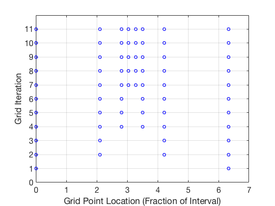
Adaptive mesh

We saw in our example that the accuracy of solution can be improved by adding more points to our grid. However, this technique results in significantly large number of points being added. More importantly, most of these points were added in region where the control from optimizer matched the optimal control value. Adaptive meshing can be used to improve the accuracy of the solution. The effect of this adaptive process can be seen below,

Fig 7. Control obtained using adaptive mesh.

Note, more grid points are located closer to the point where control switches from -1 to 1. This adaptive change in grid location can be seen in the plot below.

Fig 8. Different iterations grid points for obtained using adaptive mesh.

6. GPOPs II

GPOPs II (pronounced GPOPs 2) is a general purpose optimal control software. GPOPs II stands for, General Purpose OPtimal Control Software version 2. GPOPs’ development began in 2007, and the development of GPOPS-II continues today, with improvements that include the open-source algorithmic differentiation package ADiGator and continued development of $hp$-adaptive mesh refinement methods for optimal control. Detailed article on GPOPS II and its capibilites can be found here

GPOPs II was originally developed for space applications, such as planning interplanetary trajectories, satellite orbit change, etc. Over the past few years, it has found it has been extensively applied for several aerospace, robotic manipulators, walking robots, autonomous vehicles, and control of chemical plants. Here a quick introduction to GPOPS II software is provided.

** GPOPS II is available for free to all the students in MEC 560 class, please use the links provided on blackboard to download and install GPOPS II. The current license is valid until December 2016. Mechanical Engineering department at stony brook has acquired a license for the entire department. Also, please install ADiGator, an opensource software used to compute derivatives of userdefined MATLAB functions. **

A typical problem setup for GPOPS II looks as follows,

1. Define bounds on all the variables

First task is to define the bounds on multiple variables. GPOPS II provides the ability to define multiphase models, this allows us to derive optimal control for complex behaviors where the model may change during operation. Walking robots, batch reactors and multi-stage rockets are a few examples. The bounds on variables are specified using the bound stuct variable.

%-------------------------------------------------------------------------%
%----------------- Provide All Bounds for Problem ------------------------%
%-------------------------------------------------------------------------%
t0min = 0;  t0max = 0;
tfmin = 0;  tfmax = 200;
x10   = +10; x1f   = 0;
x20   = +0; x2f   = 0;
x1min = -20; x1max =  20;
x2min = -20; x2max =  20;
umin = -1;   umax = +1;

%-------------------------------------------------------------------------%
%----------------------- Setup for Problem Bounds ------------------------%
%-------------------------------------------------------------------------%
bounds.phase.initialtime.lower = t0min;
bounds.phase.initialtime.upper = t0max;
bounds.phase.finaltime.lower = tfmin;
bounds.phase.finaltime.upper = tfmax;
bounds.phase.initialstate.lower = [x10, x20];
bounds.phase.initialstate.upper = [x10, x20];
bounds.phase.state.lower = [x1min, x2min];
bounds.phase.state.upper = [x1max, x2max];
bounds.phase.finalstate.lower = [x1f, x1f];
bounds.phase.finalstate.upper = [x1f, x1f];
bounds.phase.control.lower = [umin];
bounds.phase.control.upper = [umax];

2. Provide initial guess to the solver

In GPOPs II (or any nonlinear programming), the the number of parameters can become very large, therefore it is important to provide good initial guess. A good choice of initial guess is a linear fit between the start and final desired states.

%-------------------------------------------------------------------------%
%---------------------- Provide Guess of Solution ------------------------%
%-------------------------------------------------------------------------%
tGuess               = [0; 5];
x1Guess              = [x10; x1f];
x2Guess              = [x20; x2f];
uGuess               = [umin; umin];
guess.phase.state    = [x1Guess, x2Guess];
guess.phase.control  = [uGuess];
guess.phase.time     = [tGuess];

We next define the mesh (grid) and mesh refinement method. $hp$-method is an adaptive scheme which progressively adds grid points to improve the accuracy of the optimizer.

%-------------------------------------------------------------------------%
%----------Provide Mesh Refinement Method and Initial Mesh ---------------%
%-------------------------------------------------------------------------%
mesh.method          = 'hp-PattersonRao';
mesh.tolerance       = 1e-6;
mesh.maxiterations    = 20;
mesh.colpointsmin    = 4;
mesh.colpointsmax    = 10;
mesh.phase.colpoints = 4;

4. Set up the problem

The problem is set up by specifying the dynamics and constraints for the dynamic system we intend to derive the controller for. In addition to the dynamics, we need to specify the specific solver to use. The solver we use (almost always) with GPOPS II is ipopt. The next 3 options specify the method to compute derivative during optimization. More details on derivative computation can be found here.

%-------------------------------------------------------------------------%
%------------- Assemble Information into Problem Structure ---------------%        
%-------------------------------------------------------------------------%
setup.mesh                        = mesh;
setup.name                        = 'Double-Integrator-Min-Time';
setup.functions.endpoint          = @doubleIntegratorEndpoint;
setup.functions.continuous        = @doubleIntegratorContinuous;
setup.displaylevel                = 2;
setup.bounds                      = bounds;
setup.guess                       = guess;
setup.nlp.solver                  = 'ipopt';
setup.derivatives.supplier        = 'sparseCD';
setup.derivatives.derivativelevel = 'second';
setup.method                      = 'RPM-Differentiation';

Dynamics of double integrator

function phaseout = doubleIntegratorContinuous(input)

t  = input.phase.time;
x1 = input.phase.state(:,1);
x2 = input.phase.state(:,2);
u  = input.phase.control(:,1);

x1dot = x2;
x2dot = u;

phaseout.dynamics = [x1dot, x2dot];

Objective for cost function

function output = doubleIntegratorEndpoint(input)

output.objective = input.phase.finaltime;

4. Solve the problem using GPOPS II

The GPOPS II solver can be called using simple gpops2 command as follows.

%-------------------------------------------------------------------------%
%----------------------- Solve Problem Using GPOPS2 ----------------------%
%-------------------------------------------------------------------------%
output = gpops2(setup);

Solution from GPOPS II

Using GPOPS II, we get the solution for state and control as,

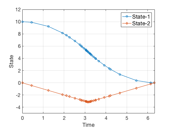
Fig 9. States for optimal control computed using GPOPS II.

Fig 10. Control for optimal control computed using GPOPS II.

Figures above show that the solution from GPOPS II is more accurate than the solution from direct collocation alone, and this solution is obtained using much fewer points.

Practial tips for optimization

It is important to frame the nonlinear programming problem appropriately. An illposed over-constraint problem can result in poor convergence properties, below are some tips on designing a well-posed nonlinear program.

Cost function: It is important to define cost functions that have smooth derivatives. This greatly simplifies the search space and makes slope calculations easier. If the cost function is not smooth, it can be made smooth by modifying the cost function. For example, $ abs( x ) $ can be written as $ \sqrt{X^2 + \epsilon } $ or cost function can be expresses as $ x $ with the constraint that $ x \geq 0 $.
Initial guess: Initial guess is the most important user-specified input to optimization routines. A good initial guess puts the solver in region of global minima and avoids potentially getting stuck in local minimas. However, it is not always possible to compute a good initial guess. In most cases, the following tricks give a good initial guess,
- Initialize states as linear functions between start and end
- Solve the problem for a simpler kinematic model by completely ignoring the dynamics of the plant.
- Solve a simpler problem with simpler cost function first, and then use it as initial guess for the main problem. For example, power is a complex cost function $ abs(u \dot{x}) $, therefore instead a quadratic cost function can be defined first $ u^2 $, and the solution from this simpler problem can be used as initial guess in the next stage.
- Solve optimization with a small grid size, and use this as input for finer or more advanced mesh types.
- Solve optimization with fewer constraints first, and then solve the full problem with all the constraints included.
- Use experimental data or domain knowledge to specify the initial guess. For example, in human reaching tasks, a minimum jerk trajectory can be a good initial guess for the optimizer.
Bound constraints: Typically as more bound contraints are included, the solver’s search space narrows, and an approximate solution can be found.
Path contraints: Path constraints refer to constraints that are applied between the final and initial time, and cannot be expressed as bounds on the state or control variables. For example, in walking the constraint that foot never crosses the ground. Such constraints can significantly restrict the search space, and lead to infeasible solutions. One way to fix this is to first compute a sub-optimal trajectory with fewer path constraints, and then add path constraints with this trajectory as initial guess.
Derivatives: Almost all optimization softwares’ performance significantly improves if analytical derivatives of cost function and constraint functions are provided. However, in some cases computing these derivatives is not easy, in such cases in custom scripts can be used to modify the derivative functions. ADiGator is one such opensource tool for differentiation. Given a user written file, together with information on the inputs of said file, ADiGator uses forward mode automatic differentiation to generate a new file which contains the calculations required to compute the numeric derivatives of the original user function.

Concluding remarks

In the last 2 classes we saw how to formulate optimal control problem. We derived necessary conditions that the optimal control needs to satisfy, and applied them to derive controllers for a specific case called linear quadratic regulator. We next looked into dynamic programming and shooting methods for computing optimal control, and finally went over direct collocation. We saw how to use GPOPS II to compute optimal control. There are several variations of optimal control problems, and GPOPS II is a very powerful tool to compute optimal control for such tasks.

Additional resources

There are several other toolkits available to solve the trajectory optimization problems. Two particularly useful resources are on webpage of Anil V Rao. Dr Anil V Rao is the author of GPOPS II, and provided free license for use in MEC 560 class.

For those seeking to use optimal trajectory control outside MEC 560, you may use OptimTraj. OptimTraj is an opensource optimal trajectory software that applies direct collocation to solve nonlinear programming problems using MATLAB’s fmincon. OptimTraj is written by Dr Matthew P. Kelly. Dr Matthew Peter Kelly has done a lot of work in control of biped robots using direct collocation for trajectory optimization. A concise introduction to direct collocation can be found in this youtube video and tutorial here.