Nonlinear control systems: Introduction and Analysis

Vivek Yadav, PhD

Introduction to nonlinear systems and their behavior

Almost all systems are nonlinear in nature. In most cases the system can be approximated by a simpler linear model, and in most cases the effects of nonlinearities are small and can be ignored. However, this is not always possible. Depending on the type of nonlinearity, the states of the system can show convergent, divergent or cyclic behavior. Examples below illustrate these concepts with a few simple examples.

Consider a simple example of underwater vehicle,

$\ddot{x} = u - \dot{x} |\dot{x}|$

the \( \dot{x}

\dot{x}

\) term represents the drag due to water.

We will study the special case when the control input $ u = 0 $. The unforced system is now given by

$\ddot{x} = - \dot{x} | \dot{x} |$

This system has negative derivative when $\dot{X}>0$ and positive derivative when $\dot{X}<0$. Therefore, the rate at which the system’s states are growing is always reducing, thus resulting in a case where the system is always stable. Such nonlinearities are also called dissipative or stabilizing nonlinearities.

This however is not necessarily the case. We may have a nonlinearity that can make the states of the system unstable. Consider the system below,

$\ddot{x} = u - x^2$

In the example above if the states of the system start with a positive value then the gradient is negative and the states of the system reduce to zero. However, if the initial value of $ x $ is negative, then the gradient is a negative number and the state goes to minus infitity. In this case the nonlinearity is non-dissipative or destabilizing.

Therefore, depending on the type of nonlinearity a system can become stable or unstable. Nonlinear systems exhibit another interesting property where the states of the system can undergo a periodic motion, and never converge to a fixed value nor diverge to infinity.

Van der pol oscillator

An extensively studied second order nonlinear system is the Van der Pol oscillator. The Van der Pol oscillator has the form,

$\ddot{X} + u(X) \dot{X} + V(X) = 0$

where, $ u(X)$ and $ V(X) $ can be considered nonlinear analogs of viscosity and stiffness. Consider the special case where,

$\ddot{X} - \mu (1- X^2) \dot{X} + X = 0$

The equation above can be expressed in state space form using,

$\dot{X_1} = X_2$ $\dot{X_2} = \mu (1- X_1^2) X_2 - X_1$

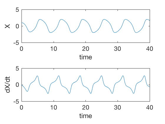
where $ \mu $ is a damping parameter. A good way to visualize the behavior of nonlinear systems is to plot one state vs other, typically a variable vs its derivative. These diagrams are referred as phase plots.

clc
close all
clear all

mu = 1;

sys_vanderPol = @(t,X)[X(2);mu*(1-X(1)^2)*X(2) - X(1)];

X0 = [1;0];
time_span = 0:.1:40;

[time,states] = ode45(sys_vanderPol,time_span,X0);

figure;
subplot(2,1,1)
plot(time,states(:,1))
xlabel('time')
ylabel('X')
subplot(2,1,2)
plot(time,states(:,2))
xlabel('time')
ylabel('dX/dt')

figure;
plot(states(:,1),states(:,2));
xlabel('X');
ylabel('dX/dt');

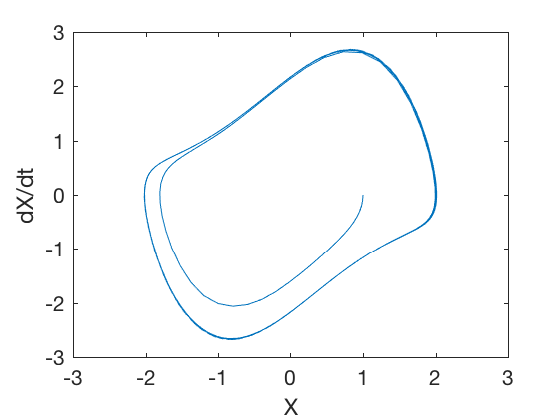
Figure below presents phase plots for different initial conditions. Regardless of the initial condition, the states converge into a periodic cycle. This periodic cycle is referred as a limit cycle.

Therefore, in addition to states going to a fixed value and diverging to infinity, the states can exhibit a periodic behavior called limit cycle. A certain class of differential equations that exhibit such periodic behavior are called Lienard systems.

Lienard systems

Consider the differential equation below,

$y_1 = f_1(t,X)$ $y_2 = f_2(t,X)$

if for some $f_1$ and $f_2$, we have

$\frac{\partial f_1}{\partial t} + \frac{\partial f_2}{\partial t} \neq 0$

then the limit cycle does not exist. The the left hand side expression is zero, then a limit cycle may exist. For a special class of Lienard systems that can be expressed as

$\ddot{X} + F'(X) \dot{X} + G'(X) = 0,$

Lienard theorm for limit cycles

Lienard theorm states that if we have two smooth odd functions F and G’ such that G’(X) > 0 for X > 0 and such that F has exactly three zeros 0, a, −a with F’(0) < 0 and F’(X) ≥ 0 for X > a and F(X) → ∞ for X →∞. Then the corresponding Lienard system has exacactly one limit cycle and this cycle is stable.

Note the expression above states that the the derivative of F increases if the X is above 0 and descreases if X is greater than a. This results in a case where states of the system diverge away from 0, and instead of converging to a fixed value, converge to a periodic orbit.

By choosing,

$F(X) = \mu \left( \frac{X^3}{3}-X \right)$

and

$G(X) = \frac{X^2}{2},$ $\ddot{X} + F'(X) \dot{X} + G'(X) = 0$

becomes,

$\ddot{X} - \mu \left( 1 - X^2 \right) \dot{X} + G'(X) = 0$

which is the equation of Van der Pol oscillator.

Therefore, based on the type of nonlinearity and initial conditions a system’s states may diverge, go to a fixed point or go into a periodic motion called limit cycle. Therefore, formal techniques are developed to study properties of nonlinear system.

Techniques for stability analysis of nonlinear systems.

Nonlinear systems can exhibit stability in two modes. They may either have an equilibirum point to which states converge, or have a limit cycle where states undergo a periodic motion.

1. Equiliribum point

Consider the system given by

$\dot{X} = f(X)$

A point $ X_{eq} $ is called equilibirum point if

$f( X_{eq}) = 0$

However, this equilibirum point need not be stable. If in the neighborhood of $X_{eq}$, the direction of derivative is away from it, the states move away.

2. Limit cycle

Limit cycle as shown above are periodic orbits that the states of a nonlinear system settle into. Limit cycles are useful property to exploit in applications where the objective is to obtain periodic motion. Limit cycles are typically difficult to find. Limit cycles can be stable, unstable or half stable. Half stable limit cycles are limits cycles that are stable for initial values inside the region enclosed by limit cycle, and unstable outside. Consider the example of a simple system given by,

$\dot{r} = (r^2-1)$ $\dot{\theta} = 1$

In the above equations, if \(

< 1 \), then states diverge until $ r = 1 $. But for $ r > 1 $, the states go to infinity. The phase plot for such a system in cartesian coordinates are given by

Therefore, unlike linear systems, stability of nonlinear systems depends on the nature of nonlinearity and the state of the system. Therefore eigen value analysis methods developed for the linear systems cannot be applied directly. Three techniques used to determine if a system is stable are,

Solve the differential equations, either numerically (simulations) or analytically and study the behavior of the solution.
Linearize the nonlinear system about some operating point and study its behavior, however, this method is susceptible to linearizing errors.
Define a Lyapunov function and study the behavior of the function itself.

Of all the methods described above, the Lyapunov approach is the most veratile, and is most used for analysis of nonlinear systems.

Lyapunov method for Nonlinear system analysis

In Lyapunov method, we define a positive-definite function, $ L $, take its derivative with respect to time and study its behavior. We choose Lyapunov function in such a way that it is zero at the equilibrium point we are investigating. The Lyapunov method can be described as follows,

Define a Lyapunov function $ L $ that is positive definite for all points in the space except the equilibrium point.
Compute the derivative of the Lyapunov function, and check if its properties.
- If the Lyapunov function is always negative, then states go to the equilibrium point asymptotically.
- If the Lyapunov function is neagative for all $ X > a $ for some $ a $, then $ a $ represents the stability boundary i.e. after infitite time states will be bounded by $ a $ for all time.

Lyapunov method for continuous systems

We will next apply Lyapunov method to study behavior of Van der Pol oscillator. Consider the system given by,

$\dot{X_1} = X_2$ $\dot{X_2} = \mu (1- X_1^2) X_2 - X_1$

We formulate a Lyapunov function as,

$L(X_1,X_2) = \frac{1}{2} X_1^T X_1 + \frac{1}{2} X_2^T X_2$

Taking derivative of the Lyapunov with respect to time gives,

$\frac{ \partial L }{ \partial t} = X_1^T \dot{X}_1 + X_2^T \dot{X}_2$

Substituting derivatives from state equation gives,

$\frac{ \partial L }{ \partial t} = X_1^T X_2 + X_2^T \left( \mu (1- X_1^2) X_2 - X_1 \right)$ $\frac{ \partial L }{ \partial t} = \mu X_2^T (1- X_1^2) X_2$

Note $ \mu = 0 $, is a special case where the Lyapunov function does not change and the system exhibits a fixed periodic motion. We will focus on other two cases, where $ \mu >0 $ and $ \mu < 0 $.

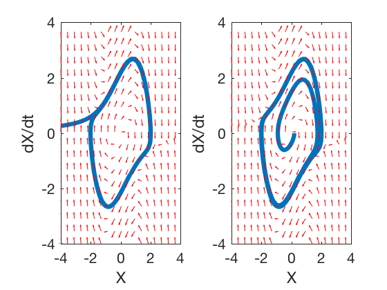
1. $ \mu > 0 $

In this case, we simply replace $ \mu $ by \(

\mu

\), as this does not change the behavior of the system. The Luapunov now becomes,

$\frac{ \partial L }{ \partial t} = |\mu| X_2^T (1- X_1^2) X_2$

Therefore if $ 1 - X_1^2 < 0 $ the Lyapunv function will decrease, therefore the state variables will always remain bounded. If $ (1 - X_1^2) > 0 $, the states of the system go towards $ X_1^2 = 1 $.

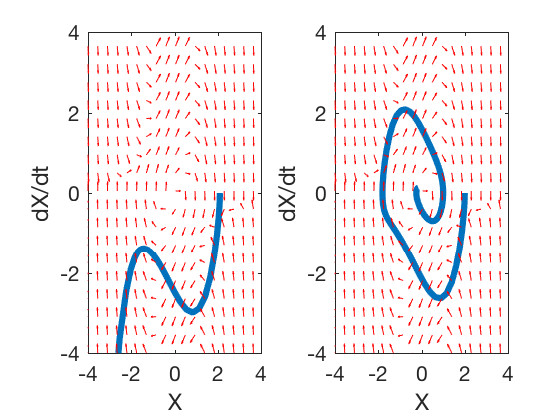
2. $ \mu < 0 $

In this case, we replace $ \mu $ by \( -

\mu

\), as this does not change the behavior of the system. The Luapunov now becomes,

$\frac{ \partial L }{ \partial t} = - |\mu| X_2^T (1- X_1^2) X_2$

Therefore if $ (1 - X_1^2) > 0 $ the states of the systems converge to zero, and if $ (1 - X_1^2) < 0 $ the states of the system go to infinity.

Therefore, by using Lyapunov method, we could describe the behavior of the system for different parameter values and different state values.

** Note: For discrete systems, the Lyapunov function is defined similarly as the continuous case, but stability is investigated by taking difference in this cost between current Lyapunov function value and previous Lyapunov function value. We will look into more examples of Lyapunov function in the coming classes. **

clc
close all
clear all

X1_0 = -4:.45:4;
X2_0 = -4:.45:4;

[X1_0,X2_0] = meshgrid(X1_0,X2_0);
mu = 1;
sys_vanderPol = @(t,X)[X(2);mu*(1-X(1)^2)*X(2) - X(1)];

X0 = [X1_0(1);X2_0(1)];
time_span = 0:.1:40;

[time,states] = ode45(sys_vanderPol,time_span,X0);
[time,states1] = ode45(sys_vanderPol,time_span,[.2;0]);

dX1  = X2_0;
dX2  = (1-X1_0.^2).*X2_0 - X1_0;
dX1 = dX1./sqrt(dX1.^2+dX2.^2);
dX2 = dX2./sqrt(dX1.^2+dX2.^2);

figure;
subplot(1,2,1)
plot(states(:,1),states(:,2),'linewidth',3)
hold on
quiver(X1_0,X2_0,dX1,dX2,.5,'r')
axis([-4 4 -4 4])
xlabel('X');
ylabel('dX/dt');
subplot(1,2,2)
plot(states1(:,1),states1(:,2),'linewidth',3)
hold on
quiver(X1_0,X2_0,dX1,dX2,.5,'r')
axis([-4 4 -4 4])
xlabel('X');
ylabel('dX/dt');

clc
close all
clear all

X1_0 = -4:.45:4;
X2_0 = -4:.45:4;

[X1_0,X2_0] = meshgrid(X1_0,X2_0);
mu = -1;
sys_vanderPol = @(t,X)[X(2);mu*(1-X(1)^2)*X(2) - X(1)];

time_span = 0:.1:10;

[time,states] = ode45(sys_vanderPol,time_span,[2.1;0]);
[time,states1] = ode45(sys_vanderPol,time_span,[2;0]);

dX1  = X2_0;
dX2  = (1-X1_0.^2).*X2_0 - X1_0;
dX1 = dX1./sqrt(dX1.^2+dX2.^2);
dX2 = dX2./sqrt(dX1.^2+dX2.^2);

figure;
subplot(1,2,1)
plot(states(:,1),states(:,2),'linewidth',3)
hold on
quiver(X1_0,X2_0,dX1,dX2,.5,'r')
axis([-4 4 -4 4])
xlabel('X');
ylabel('dX/dt');
subplot(1,2,2)
plot(states1(:,1),states1(:,2),'linewidth',3)
hold on
quiver(X1_0,X2_0,dX1,dX2,.5,'r')
axis([-4 4 -4 4])
xlabel('X');
ylabel('dX/dt');

More examples.

Consider the system given by,

$\dot{X}_1 = \mu - X_1^2$ $\dot{X}_2 = - X_2$

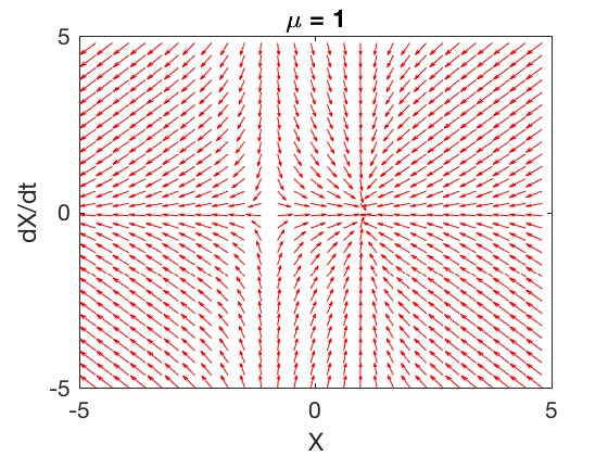
Plots below show the phase plot of the derivatives of the system above for 3 different values of $ \mu $. For $ \mu=0$, the system has 1 equilibrium point, at $ X1 = 0 $, however this point is not stable because for $ X_1 < 0 $, the derivative is negative which results in the states of the system diverging to minus infinity.

For $ \mu = -1 $, the equilibrium points do not exist, and the states go to minus infinity.

For $ \mu = 1 $, the equilibrium points are at $ X_1 = +/- 1 $ and $ X_2 = 0 $. The equilibrium point on right is more stable and the one on left is an unstable equilibrium point.

clc
close all
clear all

X1_0 = -5:.35:5;
X2_0 = -5:.35:5;

[X1_0,X2_0] = meshgrid(X1_0,X2_0);
mu = 1;
sys_SS = @(t,X)[mu - X(1)^2;-X(2) ];

time_span = 0:.1:10;

[time,states] = ode45(sys_SS,time_span,[2;1]);

dX1  = mu - X1_0.^2;
dX2  = - X2_0;
dX1 = dX1./sqrt(dX1.^2+dX2.^2);
dX2 = dX2./sqrt(dX1.^2+dX2.^2);

figure;
quiver(X1_0,X2_0,dX1,dX2,1,'r')
axis([-5 5 -5 5])
xlabel('X');
ylabel('dX/dt');
title('\mu = 1')

Graphical techniques are very useful in recognizing the behavior of the system. However, this technique applies only to system with very few states. We will focus on analytical methods that can be applied to different types of systems.