Output feedback control, Observability and Observer design

Vivek Yadav, PhD

In many applications, we are more interested in driving the measurements of the system to some desired value. For example, while designing controller for walking robot, we are more interested in the hip velocity than the involved joint angles. Therefore, in such cases, we are more interested in designing a controller that drives the output of the system to a desired value, than the actual states themselves. The field of control theory that deals with modifying the behavior of the output of the system is referred as output feedback control theory.

Consider a system given by

$\frac{d x }{dt} = A x + B u$

with measurements

$y = C x.$

We design a controller $ u = -Ky $. The system dynamics becomes,

$\frac{d x }{dt} = (A - BKC) X$

If we are able to choose a $ K $ such that the eigenvalues of $ (A - BKC) $ have negative real parts, then we can design a controller that will drive the states of the system, and hence measurements to zero. However, depending on the values of the system dynamics and measurement matrices, this may not be possible. Consider the following example.

Motivating example:

Consider the system given by,

$\dot{X} = \left[ \begin{array}{cc} 0 & 1 \\ 0 & 0 \end{array} \right] X + \left[ \begin{array}{c} 0 \\ 1 \end{array} \right] u$

with measurement

$y = \left[ \begin{array}{cc} 1 & 0 \end{array} \right] X .$

and control

$u = - Ky = - KCX$

where $ K = 1 $. The $ (A - BKC) $ matrix in this case is,

$A-BKC = \left[ \begin{array}{cc} 0 & 1 \\ 0 & 0 \end{array} \right] - \left[ \begin{array}{c} 0 \\ 1 \end{array} \right] \times 1 \times \left[ \begin{array}{cc} 1 & 0 \end{array} \right] = \left[ \begin{array}{cc} 0 & 1 \\ -1 & 0 \end{array} \right]$

The matrix above has eigen values at $ \pm j $, i.e real part zero. Therefore, the system above can not be stabilized using the control $ u = -K y $. This is also illustrated by the example below,

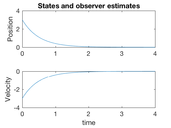
%% Observer design example

clc
close all
clear all 


A = [0 1 ; 0 0]; 
B = [0 ; 1];
C = [1 0];

X0 = [1;0];
t = 0:0.01:10;

K = 1;


sys_OFC = @(t,X)[A*X - B*K*C*X]

[t,X] = ode45(sys_OFC,t,X0);

sys_OFC = 

    @(t,X)[A*X-B*K*C*X]

figure;
subplot(2,1,1)
plot(t,X(:,1))
title('States and observer estimates')
ylabel('Position')
subplot(2,1,2)
plot(t,X(:,2))
ylabel('Velocity')
xlabel('time')

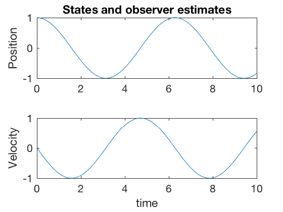
It can be shown that for all real-values of $ K $, the system has eigen values with zero real parts. Therefore, it is not possible to drive the states of the system to zero. However, we saw in earlier classes that the states could be sent to zero if velocity information is incorporated. Oberverbaility and observer design concepts can be used to extract various states of a system. In this example, velocity from position.

Observability and observer design

In previous classes we saw how to use pole-placement and optimal control techniques to design controllers for linear system under various constraints. One limitation of previous techniques was that we assumed that full-state information was available for us for design. However, we monitor a system using its measurements, and these measurements need not be the complete state vector. In most applications, the state vector is estimated based on measurements from the plant. This can be formally described as follows. Consider the system,

$\frac{d x }{dt} = A x + B u$

with measurements

$y = C x + Bu.$

The objective of the observer is obtain an estimate $ \hat{x} $ of the states $ x $ such that $ (x - \hat{x} $ is as small as possible. Before getting into observer design, we investigate the concepts of observability and detectability.

Observability

Concepts of observability are analogous to concepts of controllability. Observability is used to determine given the set of measurement variables, can we estimate the states of the system. An unforced system is said to be observable if for a given if and only if it is possible to determine the initial state x(0) by using only a finite history of measurements $ y( \tau)$ for $0\leq \tau \leq T $ for any time $ T $.

Observability of a continuous linear system

An unforced linear system is given by

$\frac{d x(t) }{dt} = A x(t),$

and

$y(t) = C x(t),$

Taking successive derivatives of the measurement,

$\begin{array}{c} \dot{y}(t)= C \dot{x}(t) = CA x_0 ,\\ \ddot{y}(t)= CA \dot{x}(t) = CA^2 x_0 ,\\ \vdots \\ y^{(n-1)}(t)= C A^{n-2} \dot{x}(t) = CA^{n-1} x_0 ,\\ \end{array}$

We therefore have

$\left[ \begin{array}{c} y(t)\\ \dot{y}(t)\\ \vdots \\ y^{(n-1)}(t)\\ \end{array} \right] = \underbrace{\left[ \begin{array}{c} C \\ CA \\ \vdots \\ CA^{n-1} \\ \end{array} \right]}_{observability~matrix} x_0.$

It is possible to solve for $x_0$ for a given measurement history only if the observability matrix is of rank $n$.

Observability of a discrete linear system

An unforced discrete linear system is given by

$x[k+1] = A x[k],$

and

$y[k] = C x[k],$

Taking successive values of the measurement,

$\begin{array}{c} y[0] = C x[0] ,\\ y[1] = C x[1]= C A x[0] ,\\ y[2] = C x[2]= C A^2 x[0] ,\\ \vdots \\ y[n-1] = C x[n-2]= C A^{n-1} x[0]\\ \end{array}$

We therefore have

$\left[ \begin{array}{c} y[0] \\ y[1] \\ \vdots \\ y[n-1] \\ \end{array} \right] = \underbrace{\left[ \begin{array}{c} C \\ CA \\ \vdots \\ CA^{n-1} \\ \end{array} \right]}_{observability~matrix} x[0] .$

It is possible to solve for $x_0$ for a given measurement history only if the observability matrix is of rank $n$.

Obsearvability is also expressed via a Grammian matrix Q,

$Q(T) = \int_{0}^{T} e^{ A^T \lambda } C^T C e^{A \lambda } d\lambda .$

If $ Q(T) $ is non-singular for all $ T$ then the underlying dynamic system is observable.

Only $n$ derivatives or discretizations are sufficient to determine conntrollability or observability for continuous or discrete systems because adding additional derivative or discretization equations do not increase the rank of either controllability or observability matrix.

Another form of observability matrix,

As rank of a matrix and its transpose are the same, we can use the matrix

$\left[ \begin{array}{ccccc} C^T & A^T C^T & (A^T)^2 C^T & \dots & (A^T)^{n-1} C^T \end{array} \right]$

to compute rank of the observability matrix. This matrix is the same as controllability matrix with $ A $ replaced by $ A^T $ and $ B $ replaced by $ C^T $. Observability matrix can be computed in MATLAB using ‘obsv’ command.

When do systems become unobservable?

An unobservable system is more common than uncontrollable system. A system becomes unobservable when a state variable is not measured directly and is not fed back to those state variables that are measured. Consider the following control system,

$\dot{x_1} = A_1 x_1 + B_1u$ $\dot{x_2} = A_{12} x_1 + A_{22} x_2 + B_2 u$

with measurement $y = x_1$. This system can only measure $ x_1 $. $ x_2$ cannot be measured because it does not feed into the dynamics of the measured state. It may be possible to control $ x_2 $ by applying appropriate control $ u $, design of such a control is impossible because there is no direct or indirect measure of $x_2$.

** The dynamics of a system when the measurements are zero is called zero dynamics. The states combinations that enter the zero-dynamics cannot be estimated. **

Detectability

In addition to observability, concept of stabalizability and detectability are also defined. A system is stabalizable if for any given initial conditions, there exists atleast one series of control inputs that drive the system states to 0 either in finite time or asymptotically. All controlable states are stabalizable. We say a system is detectable if the unstable states can be observed.

Observability example

Consider the system given by,

$\dot{X} = \left[ \begin{array}{cc} 0 & 1 \\ 0 & 0 \end{array} \right] X + \left[ \begin{array}{c} 0 \\ 1 \end{array} \right] u .$

with measurement

$y = C X .$

Observability matrix can be written as,

$Obs(A,C) = \left[ \begin{array}{c} C \\ C A \end{array} \right]$

We will investigate the observability of the system under 3 different conditions,

1. $ C = \left[ \begin{array}{cc} 1 & 0 \end{array} \right] $

Observability matrix in this case is,

$Obs(A,C) = \left[ \begin{array}{cc} \left[ \begin{array}{cc} 1 & 0 \end{array} \right] \\ \left[ \begin{array}{cc} 1 & 0 \end{array} \right] \left[ \begin{array}{cc} 0 & 1 \\ 0 & 0 \end{array} \right] \end{array} \right]$ $Obs(A,C) = \left[ \begin{array}{cc} 1 & 0 \\ 0 & 1 \end{array} \right]$

Rank of observability matrix is 2, so the system is measurable if we have measure of position. This is intuitive, given position, we can estimate velocity by differentiation.

2. $ C = \left[ \begin{array}{cc} 1 & 1 \end{array} \right] $

As our measurement has information on both position and velocity, we should be able to reconstruct both positions and velocity. Observability matrix in this case is,

$Obs(A,C) = \left[ \begin{array}{cc} \left[ \begin{array}{cc} 1 & 1 \end{array} \right] \\ \left[ \begin{array}{cc} 1 & 1 \end{array} \right] \left[ \begin{array}{cc} 0 & 1 \\ 0 & 0 \end{array} \right] \end{array} \right]$ $Obs(A,C) = \left[ \begin{array}{cc} 1 & 1 \\ 0 & 1 \end{array} \right]$

Rank of observability matrix is 2, so the system is measurable if we have measure of position.

3. $ C = \left[ \begin{array}{cc} 0 & 1 \end{array} \right] $

$Obs(A,C) = \left[ \begin{array}{cc} \left[ \begin{array}{cc} 0 & 1 \end{array} \right] \\ \left[ \begin{array}{cc} 0 & 1 \end{array} \right] \left[ \begin{array}{cc} 0 & 1 \\ 0 & 0 \end{array} \right] \end{array} \right]$ $Obs(A,C) = \left[ \begin{array}{cc} 0 & 1 \\ 0 & 0 \end{array} \right]$

The observability matrix has a rank of 1, therefore the system is not measurable based on velocity alone.

Observation design

Two of the simplest observers for linear systems are a full-order observer and a reduced order observer. Full-order observers are observers that estimate the entire state-space from measurements. Full order observes are easier to design and implement, however as they ignore the fact that some states are directly measured, while others are not, they are less accurate on the onset. Reduced order observes, on the other hand are more accurate because they directly compute the measured variable, and estimate the unmeasured variable. Reduced order observers are more accurate, but are computationally more complex to implement.

Full-observer design

We now design observer for the system given by,

$\dot{X} = AX + Bu$

with measurement,

$y = CX + Du .$

In the system above, we know $ y $, the control $ u $ and the actual state $ X $ is unknown that we wish to estimate. We design an observer to estimate $ X $ as

$\dot{\hat{X}} = A\hat{X} + Bu + L (y - \hat{y})$

where $ \hat{y} $ is the approximate value of measurement, and is described as

$\hat{y} = C \hat{X} + Du .$

In the system above, the goal is to choose an $L$ such that $ \hat{X} \rightarrow X $.

Observer error

Substituting expressions for $ y $ and $ \hat{y} $ in the observer equation gives,

$\dot{\hat{X}} = A\hat{X} + Bu + L (y - \hat{y})$ $\dot{\hat{X}} = A\hat{X} + Bu + L \left( CX + Du - ( C \hat{X} + Du)\right)$ $\dot{\hat{X}} = A\hat{X} + Bu + L C ( X - \hat{X})$

The error between the state and its estimate is $ e = X - \hat{X} $, therefore, substracting system dynamics from the observer equation above gives,

$\dot{X} - \dot{\hat{X}} = A( X - \hat{X} ) - L C ( X - \hat{X})$ $\dot{e} = (A - L C )e$

If we chose $ L $ such that the eigen values of $ A - LC $ have negative real parts, then $ e \rightarrow 0 $ as $ t \rightarrow \infty $. As eigen values of $ A - LC $ are the same as eigen values of $ ( A - LC )^T $,

$eig(A - LC ) = eig\left( (A - LC )^T \right) = eig(A^T - C^TL^T )$

The problem of placing poles for $ \left( A^T - C^TL^T \right) $, is same as pole-placement for $ ( A - BK ) $ in the controller design. Therefore, we can use the same method as before with $ A $ and $ B $ replaced by $ A^T $ and $ C^T $ respectively. $ L $ can be computed from $ L = K^T $.

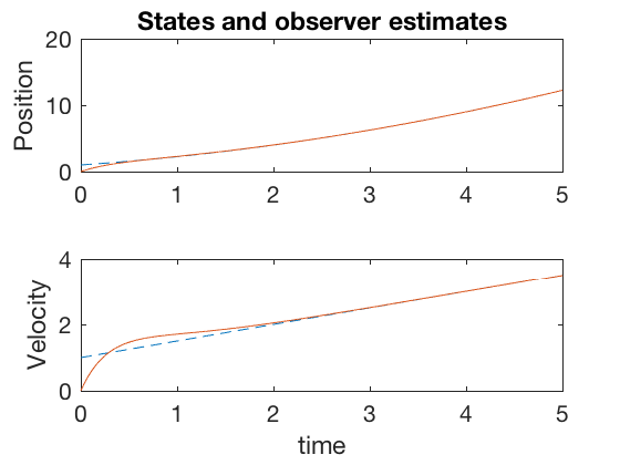
Full-order observer example

Consider the system given by,

$\dot{X} = \left[ \begin{array}{cc} 0 & 1 \\ 0 & 0 \end{array} \right] X + \left[ \begin{array}{c} 0 \\ 1 \end{array} \right] u$

with measurement

$y = \left[ \begin{array}{cc} 1 & 0 \end{array} \right] X .$

We next choose $ L $ such that eigen values of $ (A - LC) $ are -2 and -3. This technique is implemented in the code below.

%% Observer design example

clc
close all
clear all 


A = [0 1 ; 0 0]; 
B = [0 ; 1];
C = [1 0];

p = [-2;-3];

L_t = place(A',C',p);
L = L_t';
t = 0:0.001:5; 
dt = t(2) - t(1);
X(:,1) = [1;1];
y(:,1) = C*X;

X_hat(:,1) = [0;0];
y_hat(:,1) = C*X_hat;
for i = 2:length(t)
    u = .5;
    
    X(:,i) = X(:,i-1)  +dt * (A*X(:,i-1) + B*u);
    y(:,i) = C*X(:,i) ;

    X_hat(:,i) = X_hat(:,i-1)  +dt * (A*X_hat(:,i-1) + B*u +L*(y(:,i-1)-y_hat(:,i-1)));
    y_hat(:,i) = C*X_hat(:,i) ;
end

figure;
subplot(2,1,1)
plot(t,X(1,:),'--',t,X_hat(1,:))
title('States and observer estimates')
ylabel('Position')
subplot(2,1,2)
plot(t,X(2,:),'--',t,X_hat(2,:))
ylabel('Velocity')
xlabel('time')

figure;
subplot(2,1,1)
plot(t,X(1,:)-X_hat(1,:))
ylabel('Position')
title('Error: states - observer estimates')
subplot(2,1,2)
plot(t,X(2,:)-X_hat(2,:))
ylabel('Velocity')
xlabel('time')

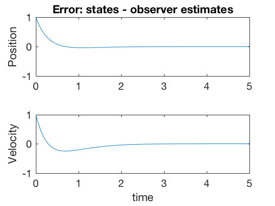
Figures above show that the states and observer estimates converge to the same values, and the error goes to zero after 2 seconds of start. If the observer estimates can be initialized so they are closer to the actual system states, then the observer estimates converge faster. However, this is not always possible nor a necessary requirement for observer estimates to converge to actual measurements.

** Important: In the plots above, the error in position estimates is not zero, inspite of the fact that we have a direct measure of position. We can get improved performance by designing our oberver to compute the position directly, and estimate velocity. This technique is implemented via reduced-observer design. **

Reduced-order observer design.

Reduced order observers directly compute the measured variable, and estimate the unmeasured variable. This technique is more accurate than the full-order observer, but is computationally more complex to implement. We now design a reduced-order observer for the system given by,

$\dot{X} = AX + Bu$

with measurement,

$y = CX + Du .$

We assume that we have a $ n$-dimensional state vector and an $ p (< n) $ dimensional measurement vector. A reduced-order observer is constructed in following steps,

1. Transform system

We aim to find a transformation $ P $ such that after transformation $ X = PZ $, the system dynamics change as

$\dot{Z} = A_z Z + B_zu$

with measurement,

$y = Z_1 + D u,$

where the new transformed state-space is

$Z = \left[ \begin{array}{c} Z_1 \\ Z_2 \end{array} \right].$

The transformation $ P $ can be found as follows,

Perform elementary column operations to find a nonsingulr matrix R of dimensions $ n \times n $ such that $ CR = \left[ \begin{array}{cc} C_1 & 0 \end{array} \right] $, where $ C_1 $ is an invertible $ p $ dimensional matrix.
Choose, $P = R \left[ \begin{array}{cc} C_1^{-1} & 0 \\ 0 & I_{n-p} \end{array} \right]$ Now
$C P = CR \left[ \begin{array}{cc} C_1^{-1} & 0 \\ 0 & I_{n-p} \end{array} \right] = [I_p 0]$

Using $ P $ above for transormation $ X = PZ $ the system,

$\dot{X} = AX + Bu$

with measurement,

$y = CX + Du .$

transforms as,

$\dot{Z} = \underbrace{P^{-1} A P}_{A_z} Z + \underbrace{P^{-1}B}_{B_z} u$

with measurement,

$y = CPZ + D u = Z_1 + Du.$

We next partition the state space,

2. Partition the state space.

Partition the state space as,

$\left[ \begin{array}{c} \dot{Z}_1 \\ \dot{Z}_2 \end{array} \right] = \left[ \begin{array}{cc} A_{z,11} & A_{z,12} \\ A_{z,21} & A_{z,22} \end{array} \right] \left[ \begin{array}{c} Z_1 \\ Z_2 \end{array} \right] + \left[ \begin{array}{c} B_{z,1} \\ B_{z,2} \end{array} \right] u$

With measurements,

$y = Z_1 + Du$

We can expand and rewrite the state space equation as,

$\dot{Z}_1 = A_{z,11} Z_1 +A_{z,12} Z_2 + B_{z,1} u$ $\dot{Z}_2 = A_{z,21} Z_1 +A_{z,22} Z_2 + B_{z,2} u$

In the partioned state space above, we have direct measure of $ Z_1 $, so we need to design measurement for $ Z_2 $ only.

3. Observer design.

We design an observer to estimate $ \hat{K}_z $ such that $ \hat{Z}_2 \rightarrow Z_2 $ as $ t \rightarrow \infty $. Consider the system given by,

$\dot{\hat{Z}}_2 = A_{z,21} Z_1 +A_{z,22} \hat{Z}_2 + B_{z,2} u + K_z \left( \dot{Z}_1 - A_{z,11} Z_1 - A_{z,12} \hat{Z}_2 - B_{z,1} u \right)$

The error dynamics between ( \hat{Z}_2 \) and $ Z_2 $ is

$\dot{Z}_2 - \dot{\hat{Z}}_2 = A_{z,21} Z_1 +A_{z,22} Z_2 + B_{z,2} u - \left( A_{z,21} Z_1 +A_{z,22} \hat{Z}_2 + B_{z,2} u + K_z \left( \dot{Z}_1 - A_{z,11} Z_1 - A_{z,12} \hat{Z}_2 - B_{z,1} u \right) \right)$ $\dot{Z}_2 - \dot{\hat{Z}}_2 = A_{z,22} (Z_2 - \hat{Z}_2) - K_z \left( \dot{Z}_1 - A_{z,11} Z_1 - A_{z,12} \hat{Z}_2 - B_{z,1} u \right)$

Substituting $ \dot{Z}_1 $ from partitioned equations gives,

$\dot{Z}_2 - \dot{\hat{Z}}_2 = A_{z,22} (Z_2 - \hat{Z}_2) - K_z \left( \left(A_{z,11} Z_1 +A_{z,12} Z_2 + B_{z,1} u \right) - A_{z,11} Z_1 - A_{z,12} \hat{Z}_2 - B_{z,1} u \right)$ $\dot{Z}_2 - \dot{\hat{Z}}_2 = A_{z,22} (Z_2 - \hat{Z}_2) - K_z \left( A_{z,12} (Z_2 - \hat{Z}_2 ) \right)$

Defining error $ e = (Z_2 - \hat{Z}_2) $,

$\dot{e} = \left( A_{z,22} - K_z A_{z,12} \right) e$

Therefore, if we choose $ K_z $ such that the poles of the resulting system have negative real parts, then the error goes to zero. Note, it can be shown that if the system $ (A,C ) $ is observable, then the system (( A_{z,22}, A_{z,12} ) \) is also observable.

Therefore, $ Z_2 $ in

$\dot{Z}_2 = A_{z,21} Z_1 +A_{z,22} Z_2 + B_{z,2} u ,$

can be estimated using

$\dot{\hat{Z}}_2 = A_{z,21} Z_1 +A_{z,22} \hat{Z}_2 + B_{z,2} u + K_z \left( \dot{Z}_1 - A_{z,11} Z_1 - A_{z,12} \hat{Z}_2 - B_{z,1} u \right)$

where

$y = Z_1 + Du$

However, the expression above, we need to compute derivative of $ Z_1 $, this can be obtaining by applying another transformation, such that

$w = \hat{Z}_2 - K_z Z_1$

Taking derivative gives,

$\dot{w} = \dot{\hat{Z}}_2 - K_z \dot{Z}_1$

Substituting for $ \dot{\hat{Z}}_2 $ gives $\dot{w} = A_{z,21} Z_1 +A_{z,22} (w +K_z Z_1) + B_{z,2} u - K_z \left( A_{z,11} Z_1 + A_{z,12} (w +K_z y) + B_{z,1} u \right)$

$\dot{w} = ( A_{z,22} - K_z A_{z,12} ) w + ( B_{z,2} - K_z B_{z,1} )u + (A_{z,21} - K_z A_{z,11} + A_{z,22} K_z - K_z A_{z,12} K_z) Z_1$

4. Final reduced-order observer

The final reduced order observer is given as,

$\dot{w} = ( A_{z,22} - K_z A_{z,12} ) w + ( B_{z,2} - K_z B_{z,1} )u + (A_{z,21} - K_z A_{z,11} + A_{z,22} K_z - K_z A_{z,12} K_z) Z_1$

The original state-space representation can be reconstructed using

$X = P Z = P \left[ \begin{array}{c} Z_1 \\ w + K_z Z_1 \end{array} \right]$

Where $ K_z $ is chosen such that

$( A_{z,22} - K_z A_{z,12})$

has negative real parts of eigen values.

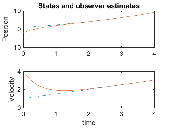
Example 1: Reduced-order observer

Consider the system given by,

$\dot{X} = \left[ \begin{array}{cc} 0 & 1 \\ 0 & 0 \end{array} \right] X + \left[ \begin{array}{c} 0 \\ 1 \end{array} \right] u$

with measurement

$y = \left[ \begin{array}{cc} 1 & 1 \end{array} \right] X .$

Solution process:

1. Transform system

In this case, as $ C $ is in the form

$\left[ \begin{array}{cc} 1 & 1 \end{array} \right] ,$

we to apply a similarity transformation. We identify that

$R = \left[ \begin{array}{cc} .5 & .5 \\ .5 & -.5 \end{array} \right] ,$

when multiplied by $ C $ gives, $C R = \left[ \begin{array}{cc} 1 & 1 \end{array} \right]\left[ \begin{array}{cc} .5 & .5 \\ .5 & -.5 \end{array} \right] = \left[ \begin{array}{cc} 1 & 0 \end{array} \right]$

where

$C_z = 1 .$

We therefore choose $ P $ as,

$P = R \left[ \begin{array}{cc} C_1^{-1} & 0 \\ 0 & I_{n-p} \end{array} \right]$ $P = \left[ \begin{array}{cc} .5 & .5 \\ .5 & -.5 \end{array} \right] \left[ \begin{array}{cc} 1 & 0 \\ 0 & 1 \end{array} \right] = \left[ \begin{array}{cc} .5 & .5 \\ .5 & -.5 \end{array} \right]$

Applying the transformation,

$X = P Z = \left[ \begin{array}{cc} .5 & .5 \\ .5 & -.5 \end{array} \right] Z$

gives,

$\dot{Z} = \underbrace{P^{-1} A P}_{A_z} Z + \underbrace{P^{-1}B}_{B_z} u$ $\dot{Z} = P^{-1} A P Z + P^{-1}B u$ $\dot{Z} = \left[ \begin{array}{cc} .5 & .5 \\ .5 & -.5 \end{array} \right]^{-1} \left[ \begin{array}{cc} 0 & 1 \\ 0 & 0 \end{array} \right] \left[ \begin{array}{cc} .5 & .5 \\ .5 & -.5 \end{array} \right] Z + \left[ \begin{array}{cc} .5 & .5 \\ .5 & -.5 \end{array} \right]^{-1} \left[ \begin{array}{c} 0 \\ 1 \end{array} \right] u$ $\dot{Z} = \left[ \begin{array}{cc} -.5 & .5 \\ -.5 & .5 \end{array} \right] Z + \left[ \begin{array}{c} -1 \\ -1 \end{array} \right] u$

And the measurement equation is,

$y = CPZ$ $y = \left[ \begin{array}{cc} 1 & 1 \end{array} \right] \left[ \begin{array}{cc} .5 & .5 \\ .5 & -.5 \end{array} \right] Z = \left[ \begin{array}{cc} 1 & 0 \end{array} \right] Z= Z_1$

2. Partition state space

We next partition the state space in the form,

$\dot{Z}_1 = A_{z,11} Z_1 +A_{z,12} Z_2 + B_{z,1} u$ $\dot{Z}_2 = A_{z,21} Z_1 +A_{z,22} Z_2 + B_{z,2} u$ $\left[ \begin{array}{c}\dot{Z}_1 \\ \dot{Z}_2 \end{array} \right] = \left[ \begin{array}{cc} .5 & -.5 \\ .5 & -.5 \end{array} \right] \left[ \begin{array}{c} Z_1 \\ Z_2 \end{array} \right] + \left[ \begin{array}{c} 1 \\ -1 \end{array} \right] u$

We get,

$A_{z,11} = .5$ $A_{z,12} = -.5$ $A_{z,21} = .5$ $A_{z,22} = -.5$

3. Choose gain for observer

We next choose $ K_z $ such that the eigen values of

$\left(A_{z,22} - K_z A_{z,12} \right)$

are at -2. This gives,

$\left(A_{z,22} - K_z A_{z,12} \right) = .5 - .5 K_z$

Therefore $ K_z = -3 $ places poles of the system at -2.

4. Final reduced-order observer

The final reduced order observer is given as,

$\dot{w} = ( A_{z,22} - K_z A_{z,12} ) w + ( B_{z,2} - K_z B_{z,1} )u + (A_{z,21} - K_z A_{z,11} + A_{z,22} K_z - K_z A_{z,12} K_z) Z_1$ $\dot{w} = -2 w + 4 u + -8 Z_1$

In expression above, we have direct measure of $ Z_1 $ so the expression above becomes,

$Z_1 = y - Du$ $Z_1 = y$ $\dot{w} = -2 w + 4 u + -8 Z_1$

The original state-space representation can be reconstructed using

$X = P Z = P \left[ \begin{array}{c} Z_1 \\ w + 5 y \end{array} \right]$

clc
close all
clear all

P = [.5 .5 ; .5 -.5];
A = [0 1 ; 0 0];
B = [0;1];
C = [1 1];

display(['Observability matrix''s rank is ' num2str(rank(obsv(A,C))) '.' ])


A_z = inv(P)*A*P;
B_z = inv(P)*B;
C_z = C*P;

p = 1;
n = size(A,1);

A_z11 = A_z(1:p,1:p);
A_z12 = A_z(1:p,p+1:n);
A_z21 = A_z(p+1:n,1:p);
A_z22 = A_z(p+1:n,p+1:n);

B_z1 = B_z(1:p);
B_z2 = B_z(p+1:n);
K_z = -3;

poles_sys = A_z22 - K_z*A_z12;
display(['Poles of the observer system are at ' num2str(poles_sys) '.' ])

A_w2 = A_z22 - K_z*A_z12;
A_wz1 = A_z21 - K_z*A_z11 + A_z22*K_z - K_z*A_z12*K_z;
B_wz = B_z2 - K_z*B_z1;

display(['Modified observer system is dw = ' num2str(A_w2) 'w +' num2str(A_wz1) 'z1 + '  num2str(B_wz) 'u' '.' ])


t = 0:0.001:4; 
dt = t(2) - t(1);
X(:,1) = [1;1];
y(:,1) = C*X;
Z_1(:,1) = y(:,1);
w(:,1) = 0;
Z_2(:,1) = K_z*Z_1(:,1)+w(:,1);
X_hat(:,1) = P*[Z_1(:,1);Z_2(:,1);];

for i = 2:length(t)
    u = .5;
    
    X(:,i) = X(:,i-1)  +dt * (A*X(:,i-1) + B*u);
    y(:,i) = C*X(:,i) ;
    
    Z_1(:,i) = y(:,i);

    w(:,i) = w(:,i-1) + dt* ( A_w2*w(:,i-1) + A_wz1*Z_1(:,i-1) + B_wz * u) ;
    
    Z_2(:,i) = K_z*Z_1(:,i)+w(:,i);
   X_hat(:,i) = P*[Z_1(:,i);Z_2(:,i);];

end

Observability matrix's rank is 2.
Poles of the observer system are at -2.
Modified observer system is dw = -2w +8z1 + 2u.

$\dot{w} = ( A_{z,22} - K_z A_{z,12} ) w + ( B_{z,2} - K_z B_{z,1} )u + (A_{z,21} - K_z A_{z,11} + A_{z,22} K_z - K_z A_{z,12} K_z) Z_1$

figure;
subplot(2,1,1)
plot(t,X(1,:),'--',t,X_hat(1,:))
title('States and observer estimates')
ylabel('Position')
subplot(2,1,2)
plot(t,X(2,:),'--',t,X_hat(2,:))
ylabel('Velocity')
xlabel('time')

figure;
subplot(2,1,1)
plot(t,X(1,:)-X_hat(1,:))
title('States and observer estimates')
ylabel('Position')
subplot(2,1,2)
plot(t,X(2,:)-X_hat(2,:))
ylabel('Velocity')
xlabel('time')

The observer estimates for both position and velocity converge to the actual state values when the measurement was their sum. Lets next investigate the case where we have measurement on position alone.

Example 1: Reduced-order observer

Consider the system given by,

$\dot{X} = \left[ \begin{array}{cc} 0 & 1 \\ 0 & 0 \end{array} \right] X + \left[ \begin{array}{c} 0 \\ 1 \end{array} \right] u$

with measurement

$y = \left[ \begin{array}{cc} 1 & 0 \end{array} \right] X .$

By following a similar process as in example before, we get,

$P = \left[ \begin{array}{cc} 1 & 0 \\0 & 1 \end{array}\right]$ $K_z = 2$

and get the evolution for $ w $

$\dot{w} = -2w -4Z_1 + u$

clc
close all
clear all

P = [1 0 ; 0 1];
A = [0 1 ; 0 0];
B = [0;1];
C = [1 0];

display(['Observability matrix''s rank is ' num2str(rank(obsv(A,C))) '.' ])


A_z = inv(P)*A*P;
B_z = inv(P)*B;
C_z = C*P;

p = 1;
n = size(A,1);

A_z11 = A_z(1:p,1:p);
A_z12 = A_z(1:p,p+1:n);
A_z21 = A_z(p+1:n,1:p);
A_z22 = A_z(p+1:n,p+1:n);

B_z1 = B_z(1:p);
B_z2 = B_z(p+1:n);
K_z = 2;

poles_sys = A_z22 - K_z*A_z12;
display(['Poles of the observer system are at ' num2str(poles_sys) '.' ])

A_w2 = A_z22 - K_z*A_z12;
A_wz1 = A_z21 - K_z*A_z11 + A_z22*K_z - K_z*A_z12*K_z;
B_wz = B_z2 - K_z*B_z1;

display(['Modified observer system is dw = ' num2str(A_w2) 'w +' num2str(A_wz1) 'z1 + '  num2str(B_wz) 'u' '.' ])


t = 0:0.001:4; 
dt = t(2) - t(1);
X(:,1) = [1;1];
y(:,1) = C*X;
Z_1(:,1) = y(:,1);
w(:,1) = 0;
Z_2(:,1) = K_z*Z_1(:,1)+w(:,1);
X_hat(:,1) = P*[Z_1(:,1);Z_2(:,1);];

for i = 2:length(t)
    u = .5;
    
    X(:,i) = X(:,i-1)  +dt * (A*X(:,i-1) + B*u);
    y(:,i) = C*X(:,i) ;
    
    Z_1(:,i) = y(:,i);

    w(:,i) = w(:,i-1) + dt* ( A_w2*w(:,i-1) + A_wz1*Z_1(:,i-1) + B_wz * u) ;
    
    Z_2(:,i) = K_z*Z_1(:,i)+w(:,i);
   X_hat(:,i) = P*[Z_1(:,i);Z_2(:,i);];

end

Observability matrix's rank is 2.
Poles of the observer system are at -2.
Modified observer system is dw = -2w +-4z1 + 1u.

figure;
subplot(2,1,1)
plot(t,X(1,:),'--',t,X_hat(1,:))
title('States and observer estimates')
ylabel('Position')
subplot(2,1,2)
plot(t,X(2,:),'--',t,X_hat(2,:))
ylabel('Velocity')
xlabel('time')

figure;
subplot(2,1,1)
plot(t,X(1,:)-X_hat(1,:))
title('States and observer estimates')
ylabel('Position')
subplot(2,1,2)
plot(t,X(2,:)-X_hat(2,:))
ylabel('Velocity')
xlabel('time')

Note in the figures above, as the measurment is the position, there is no error between estimate and state, and velocity error are lower. Further, both velocity and position go to zero within 2 seconds.

Separation principle (short for principle of separation of estimation and control)

In previous class, we discussed various methods of desinging control systems using pole-placement, dynamic programming, shooting method and direct collocation. All these methods require full estimate of the state vector. In this lesson we saw how to estimate the state variables that will be used for control. However, there is a large error between the estimates and actual values especially at the start. Therefore, it is possible that a control scheme based on observer estimates can lead to poorer performance of the entire system. Separation princple allows for the design of the controller and oberver separately, and lets us use these estimates for control. Separation principle states that under some assumptions the problem of designing an optimal feedback controller for a stochastic system can be solved by designing an observer for the state of the system, which feeds into a deterministic controller for the system. This allows us to break the problem into two separate parts, one for state estimation and one control. In practice, obersver gains are chosen such that the resulting eigen values have much larger negative real parts, than the controller. This choice drives the state estimates to states faster than the system dynamics change the system. A poorly designed observer can cause the system states to not reach the observer in a reasonable time, and can result in poorer performance while the estimates converge to the states.

Proof: Separation principle

Consider a system given by,

$\dot{X} = AX + Bu$

with measurement,

$y = CX + Du .$

with the observer model,

$\dot{\hat{X}} = A\hat{X} + Bu + L (y- C \hat{X} - Du )$

And say the control is given by,

$u = - K \hat{X}.$

We now investigate stability of the combined controller-estimator system, to do so, define the error between state and estimate,

$e = X - \hat{X}.$

Taking difference between observer and state estimate model gives,

$\dot{X} - \dot{\hat{X}} = (AX + Bu ) - (A\hat{X} + Bu + L (y- C \hat{X} - Du ))$ $\dot{e} = (A - LC ) e$

The state dynamics equation with control $ u = -K \hat{X} $ becomes,

$\dot{X} = AX + Bu = AX - BK \hat{X} = (A - BK)X +BK e$

Therefore, the complete observer-state system becomes,

$\left[\begin{array}{c} X \\ e\end{array}\right] = \left[\begin{array}{cc} (A - BK) & BK \\ 0 & (A - LC ) \end{array}\right] \left[\begin{array}{c} X \\ e\end{array}\right]$

As the combined matrix is upper triangular, the poles of the state system have no effect on the poles of the observer system.

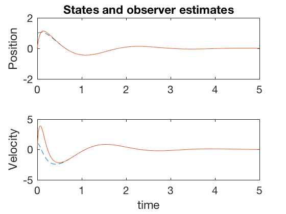
Example 1:

Consider the system given by,

$\dot{X} = \left[ \begin{array}{cc} 0 & 1 \\ 0 & 0 \end{array} \right] X + \left[ \begin{array}{c} 0 \\ 1 \end{array} \right] u$

with measurement

$y = \left[ \begin{array}{cc} 1 & 0 \end{array} \right] X .$

and control

$u = -8 \hat{X} - 2 \hat{\dot{X}}$

We design a full state observer, with poles at -10 and -15.

%% Observer design example

clc
close all
clear all 


A = [0 1 ; 0 0]; 
B = [0 ; 1];
C = [1 0];

p = [-10;-15];

L_t = place(A',C',p);
L = L_t';
t = 0:0.001:5; 
dt = t(2) - t(1);
X(:,1) = [1;1];
y(:,1) = C*X;

X_hat(:,1) = [0;0];
y_hat(:,1) = C*X_hat;
for i = 2:length(t)
    u = [-8 -2]*(X_hat(:,i-1));
    
    X(:,i) = X(:,i-1)  +dt * (A*X(:,i-1) + B*u);
    y(:,i) = C*X(:,i) ;

    X_hat(:,i) = X_hat(:,i-1)  +dt * (A*X_hat(:,i-1) + B*u +L*(y(:,i-1)-y_hat(:,i-1)));
    y_hat(:,i) = C*X_hat(:,i) ;
end

figure;
subplot(2,1,1)
plot(t,X(1,:),'--',t,X_hat(1,:))
title('States and observer estimates')
ylabel('Position')
subplot(2,1,2)
plot(t,X(2,:),'--',t,X_hat(2,:))
ylabel('Velocity')
xlabel('time')

Concluding remarks

In this lesson, we looked at some techniques to design state estimators using a technique very similar to pole placement. Analogous to linear quadratic regulator and optimal control, there exist concepts of optimal observers and estimators. We will look into these in the next class.

Output feedback control, Observability and Observer design

Vivek Yadav, PhD

Motivating example:

Observability and observer design

Observability

Observability of a continuous linear system

Observability of a discrete linear system

Another form of observability matrix,

When do systems become unobservable?

Detectability

Observability example

1. \( C = \left[ \begin{array}{cc} 1 & 0 \end{array} \right] \)

2. \( C = \left[ \begin{array}{cc} 1 & 1 \end{array} \right] \)

3. \( C = \left[ \begin{array}{cc} 0 & 1 \end{array} \right] \)

Observation design

Full-observer design

Observer error

Full-order observer example

Reduced-order observer design.

1. Transform system

2. Partition the state space.

3. Observer design.

4. Final reduced-order observer

Example 1: Reduced-order observer

Solution process:

1. Transform system

2. Partition state space

3. Choose gain for observer

4. Final reduced-order observer

Example 1: Reduced-order observer

Separation principle (short for principle of separation of estimation and control)

Proof: Separation principle

Example 1:

Concluding remarks