Control and estimation under uncertainity

Vivek Yadav, PhD

In previous lessons we saw how to design controllers and observers for dynamic systems. The extensively used pole-placement for control, observer design or linear quadratic regulators, all require information about the dyanmics of the system. However, it is not possible to accurately estimate the dynamics of a system. For example, while modeling an real system (say robot), several simplying assumptions are made, that need not be true. The mass of individual link, the location of center of mass, link lengths, moment of inertia, are all estimated using idealized assumption, and are prone to measurement errors. Another source of uncertainity is modeling error, where a physical phenomena, such as friction, may completely be ignored. These uncertainities can result in incorrect control calculations and state estimates that adversely affect the performance of the system.

Types of uncertainities

We next define different types of uncertainities formally. Consider the system that we model as,

$\dot{X} = AX + Bu$

with measurements

$Y = CX.$

Note, the representation above is what we expect the model to be, however the actual system may be different from the model above, based on the type of uncertainity. We will classify uncertainities into four broad category.

Parametric uncertainity: Parametric uncertainity refers to error in parameters that characterize a model. For example in $ F = Ma $, the model is characterized by the parameter $ M $. In cases where there is error in parameter, the actual model can be written as,

$\dot{X} = (A+ \Delta A) X + (B + \Delta B) u$ with measurements, $y = (C+ \Delta C) X$
Actuator uncertainity: Actution uncertainity comes from the fact that the control we command need not be actually applied by the actuator. Such error can be modeled as, $\dot{X} = A X + B ( u + \delta u)$ with measurements, $y =C X$
Modeling uncertainity: Modeling uncertainity refers to errors intorduced due to modeling it self. For example, phenomena such as friction, errors due to linearization, etc fall in this category. $\dot{X} = A X + B u + f(X,u)$ with measurements, $y =C X +g(X,u)$
Measurement uncertainity: Measurement uncertainity refers to errors in measurements introduced due to errors in sensor or measurement devices etc.
$\dot{X} = A X + B u$ with measurements, $y =C X + \nu$

We will look at 2 approaches to control of systems with uncertainity. The first technique assumes that the disturbance is Gaussian in nature, while the second is based on minimizing the system’s response to external disturbance. These techniques can be classified into two broad categories as follows,

1. Model uncertainity as gaussian process

Kalman filter: Kalman filters are observer analogs of linear quadratic regulators. In fact, Kalman filters are also known as linear quadratic estimators. Kalman filters does not require the uncertainity to be a gaussian process. However, if the uncertainity is gaussian in nature, then kalman filters are optimal filter in cases when the uncertainity is a gaussian process.
LQG control: LQG control stands for linear quadratic gaussian control, and is a combination of linear quadratic estimator (kalman filter) and a linear quadratic regulator.

2. Choose control to minimize sesitivity to errors.

H2 control: In H2 control, the H2 norm (root mean square of frequency response) of the system for a given disturbance is minimized, i.e. the control is designed in such a way that the sensitivity of the system measured as H2-norm is minimized.
H-$ \infty $ control: H-$ \infty $ norm refers to the largest magnitude of response to applied disturbance. In H-$ \infty $ control, the control is chosen to minimize the H-$ \infty $ norm of the response.

Kalman filter

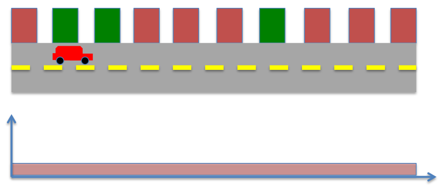
We will first look into Kalman filtering, and extend the idea for optimal control for systems with undertainities. Kalman filters combine information about system dynamics and previous measurements to estimate the current states of the system, and typically perform better than having either system dynamics or measurements alone. This is illustrated by an example, consider estimating the position of a car moving along a straight line with a constant velocity. There may be errors in orientation of the steering, difference between actual and desired velocity of the car, and in measurements obtained from the car. These errors introduce ambiguity in location of the car. If we assume the position and velocity of the car to follow a gaussian process, we can identify the region in which we expect the car to be. This is illustrated by the example below,

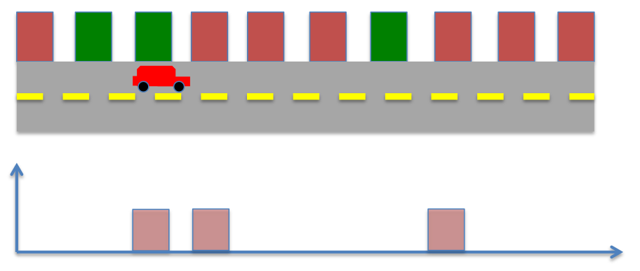
The position estimate of the car is given by the red cloud. We know approximate position and velocity at the start, as the car moves, errors are introduced due to to inaccruarate speed tracking, steering angle errors, actuation errors, etc all of which reduce our confidence in accurately locating the car and add to uncertainity. Therefore, as the car moves, the possible region where the car could be increases. However, once we get the position measurement, we can update the location of the car. However, the measurement itself is not accurate, and has some uncertainity associated with it. Therefore, the location of the car can only be estimated within a given region.

Probability: Quick review

Kalman filters are based on the idea of Baysein inference. Bayesian inference is a statistical method in which probability of an hypothesis being true is successively updated as more evidence or information becomes available. Bayesian inference is based on Bayes theorem, which gives probability of an event based on features that may be related to an event. For example, if amnesia is related to age, then, using Bayes’ theorem, a person’s age can be used to predict the probability that a person has cancer. Bayes theorm relates predictors (age) to probabilities of the hypothesis (amensia) being true. The Bayes rule can be written as,

$P(A|B) = \frac{P(B|A) P(A)}{P(B)}.$

Note the event B given A or the event A given B happens only when both A and B happen. So the Bayes rule is also sometimes written as,

$P(A|B)P(B) = P(B|A) P(A) = P(A \cap B)$

Another way to write the expression above is,

$P(A|B) = \frac{P(B|A) P(A)}{P(B|A) P(A) + P(B| \neg A) P(\neg A)} ,$

where $ \neg A $ stands for not A event.

If the event $ A $ can take multiple values say $ A_i $ for $ i : 1 \rightarrow N $.

$P(A|B) = \frac{P(B|A) P(A)}{ \sum_{i=1}^N P(B|A_i) P(A_i) } ,$

We will illustrate Bayes rule using the following 2 examples.

Example 1: Cancer testing

Say we have a test for cancer that is 99% accurate, i.e. given a person has cancer, the test gives a positive test 99% of the time. This is also referred as the true-positive rate or sensitivity. Further, if a person does not have cancer, the test gives a negative result 98% of the time, or the true negative rate/specificity is 98%. Knowing that cancer is a rare disease, and only 1.5% of the population has it, if the test comes back positive for some individual, what is the probaility that the individual actually has cancer?

Solution:

We wish to determine \( P(C

+) \), where C stands for cancer, NC stands for no cancer, - stands for negative test result, and + stands for a positive test result. The given information about cancer and test can now be written as,

Sensitivity = 99%, therefore, $ P( + C ) = .99$.
Specivity = 98%, therefore, $ P( - NC ) = .98$.
Probability of cancer = 0.015, $ P(C) = 0.015 $.

Using Bayes rule,

$P(C|+) = \frac{P(+|C) P(C)}{P(+|C) P(C) + P(+| NC) P(NC)} ,$

In expression above, we do not know \( P(+

NC) \) and $ P(NC) $. However, as

$P(+| NC) = 1 - P(-| NC) = 1 - .98 = 0.02$ $P(NC) = 1 - P(C) = 1 - .015 = 0.985$

Therefore, we can now compute probability of cancer given a positive test is,

$P(C|+) = \frac{.99 \times 0.015}{.99 \times 0.015 + .02 \times 0.985} = 0.43.$

Therefore, although the test is 99% sensitive and 98% specific, a positive results indicates about 43% chance of cancer because of low prevalance of the disease.

Example 2: Baysean estimation

Bayes’ rule can also be applied to probability distributions. Probability distributions come into play when the event cannot be approximated as a singular quantity, and has several possible states it can be in.

Scenario 1

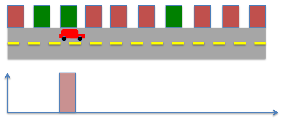
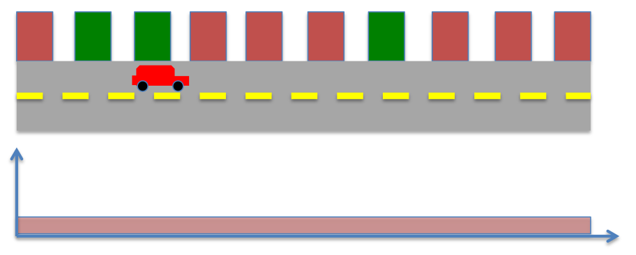
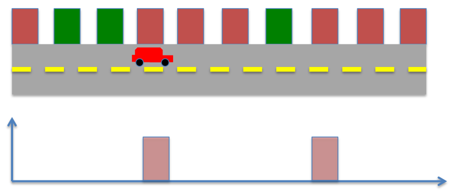
Consider a robot moving along the road as shown in the image below. We know the locations of buildings (red or green) in the world, and have sensors to detect the color of the building adjacent to the robot. Say we do not know anything to begin with, so all locations are equally likely (1/10).

$P(X)^- = \left[ \begin{array}{cccccccccc} 0.1 & 0.1 & 0.1 & 0.1 & 0.1 & 0.1 & 0.1 & 0.1 & 0.1 & 0.1 \end{array} \right]$

This probability is also called prior probability, which refers to probability before making a measurement. Further, say the robot senses either green or red, and has perfect sensor measurement. Therefore, the probability of measuring green is given by,

$P_g(X)= P(g|X)= \left[ \begin{array}{cccccccccc} 0 & 1/3 & 1/3 & 0 & 0 & 0 & 1/3 & 0 & 0 & 0 \end{array} \right]$

Similarly,

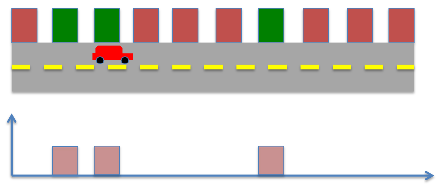
$P_r(X) =P(r|X)= \left[ \begin{array}{cccccccccc} 1/7 & 0 & 0 & 1/7 & 1/7 & 1/7 & 0 & 1/7 & 1/7 & 1/7 \end{array} \right]$

Now we sense the environment, and see a green door. The probability after measurement can be computed using Bayes’ rule. Note, probability after measurement is also referred as posteriror probability.

$P(X)^+ = P(X|g) = \frac{P(g|X)P(X)^-}{P(g)} = \frac{P(g|X)P(X)}{\sum_{i=1}^N P(g|X_i)P(X_i) }$ $P(X)^+ = P(X|g) = \frac{\left[ \begin{array}{cccccccccc} 0 & 1/3 & 1/3 & 0 & 0 & 0 & 1/3 & 0 & 0 & 0 \end{array} \right] \circ \left[ \begin{array}{cccccccccc} 0.1 & 0.1 & 0.1 & 0.1 & 0.1 & 0.1 & 0.1 & 0.1 & 0.1 & 0.1 \end{array} \right] }{\sum \left( \left[ \begin{array}{cccccccccc} 0 & 1/3 & 1/3 & 0 & 0 & 0 & 1/3 & 0 & 0 & 0 \end{array} \right] \circ \left[ \begin{array}{cccccccccc} 0.1 & 0.1 & 0.1 & 0.1 & 0.1 & 0.1 & 0.1 & 0.1 & 0.1 & 0.1 \end{array} \right] \right)}$

Where $ \circ $ operation refers to convolution operator. Convolution in this case is multiplying each element of prior probaility by the measurement probability.

$P(X)^+ = P(X|g) = \frac{\left[ \begin{array}{cccccccccc} 0 & .1/3 & .1/3 & 0 & 0 & 0 & .1/3 & 0 & 0 & 0 \end{array} \right]}{\sum \left( \left[ \begin{array}{cccccccccc} 0 & .1/3 & .1/3 & 0 & 0 & 0 & .1/3 & 0 & 0 & 0 \end{array} \right] \right)}$

The posterior probability or probability after measurement now becomes,

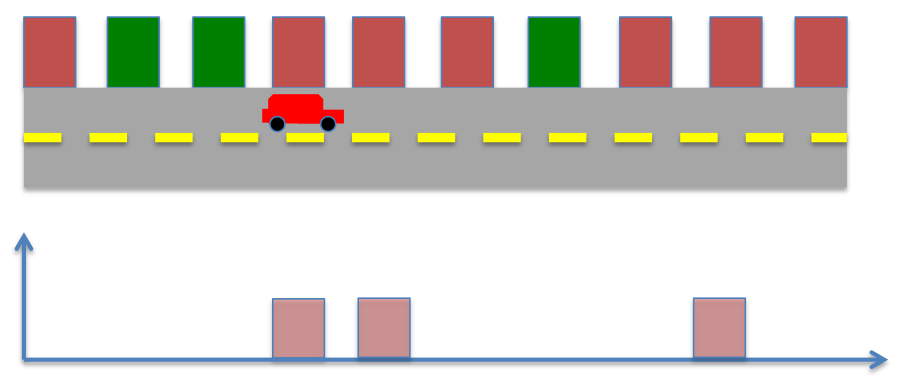
$P(X)^+ = P(X|g) = \left[ \begin{array}{cccccccccc} 0 & 1/3 & 1/3 & 0 & 0 & 0 & 1/3 & 0 & 0 & 0 \end{array} \right]$

If the robot were to stay at the same location, and keep sensing, it will measure green repeatedly, and its possible locations will not be updated. However, by moving around in the environment and sensing, the robot can get better estimate of its position. Say the robot takes 1 discrete step ahead. The possible locations of the robot and their probabilities are now given below. This probability now becomes prior probability, i.e. probability before measurement. Therefore, we relabel this probability,

$P(X)^- = \left[ \begin{array}{cccccccccc} 0 & 0 & 1/3 & 1/3 & 0 & 0 & 0 & 1/3 & 0 & 0 \end{array} \right]$

The robot now makes another measurement, and it sees its next to a green building, the measurement probability of a green building is given by,

$P_g(X)= P(g|X)= \left[ \begin{array}{cccccccccc} 0 & 1/3 & 1/3 & 0 & 0 & 0 & 1/3 & 0 & 0 & 0 \end{array} \right]$

Based on these, we can recompute the posteriror probability. From before,

$P(X)^+ = P(X|g) = \frac{P(g|X)P(X)^-}{P(g)} = \frac{P(g|X)P(X)}{\sum_{i=1}^N P(g|X_i)P(X_i) }$

Substituting prior and measurement probabilities from above,

$P(X)^+ = \frac{ \left[ \begin{array}{cccccccccc} 0 & 0 & 1/3 & 1/3 & 0 & 0 & 0 & 1/3 & 0 & 0 \end{array} \right] \circ \left[ \begin{array}{cccccccccc} 0 & 1/3 & 1/3 & 0 & 0 & 0 & 1/3 & 0 & 0 & 0\end{array} \right] }{\sum \left( \left[ \begin{array}{cccccccccc} 0 & 0 & 1/3 & 1/3 & 0 & 0 & 0 & 1/3 & 0 & 0 \end{array} \right] \circ \left[ \begin{array}{cccccccccc} 0 & 1/3 & 1/3 & 0 & 0 & 0 & 1/3 & 0 & 0 & 0\end{array} \right] \right)}$ $P(X)^+ = \frac{ \left[ \begin{array}{cccccccccc} 0 \times 0 & 0 \times 1/3 & 1/3 \times 1/3 & 1/3 \times 0 & 0\times 0 & 0\times 0 & 0\times 1/3 & 1/3\times 0 & 0\times 0 & 0\times 0 \end{array} \right] }{\sum \left( \left[ \begin{array}{cccccccccc} 0 \times 0 & 0 \times 1/3 & 1/3 \times 1/3 & 1/3 \times 0 & 0\times 0 & 0\times 0 & 0\times 1/3 & 1/3\times 0 & 0\times 0 & 0\times 0 \end{array} \right] \right)}$ $P(X)^+ = \left[ \begin{array}{cccccccccc} 0 & 0 & 1 & 0 & 0 & 0 & 0 & 0 & 0 & 0 \end{array} \right]$

Scenario 2

Consider another scenario where the robot starts in a different location as shown below. As before, we know the locations of buildings (red or green) in the world, and have sensors to detect the color of the building adjacent to the robot. As before, the probability of measuring green is given by,

$P_g(X)= P(g|X)= \left[ \begin{array}{cccccccccc} 0 & 1/3 & 1/3 & 0 & 0 & 0 & 1/3 & 0 & 0 & 0 \end{array} \right]$

and probability of measuring red is given by

$P_r(X) =P(r|X)= \left[ \begin{array}{cccccccccc} 1/7 & 0 & 0 & 1/7 & 1/7 & 1/7 & 0 & 1/7 & 1/7 & 1/7 \end{array} \right]$

As the robot does not know the position to start with, the prior probability is given by,

$P(X)^- = \left[ \begin{array}{cccccccccc} 0.1 & 0.1 & 0.1 & 0.1 & 0.1 & 0.1 & 0.1 & 0.1 & 0.1 & 0.1 \end{array} \right] .$

Now the robot senses the environment, and sees a green door. The probability after measurement can be computed using Bayes’ rule as before,

$P(X)^+ = P(X|g) = \frac{P(g|X)P(X)^-}{P(g)} = \frac{P(g|X)P(X)}{\sum_{i=1}^N P(g|X_i)P(X_i) }$ $P(X)^+ = P(X|g) = \left[ \begin{array}{cccccccccc} 0 & 1/3 & 1/3 & 0 & 0 & 0 & 1/3 & 0 & 0 & 0 \end{array} \right]$

The robot moves ahead, the prior probability now becomes,

$P(X)^- = \left[ \begin{array}{cccccccccc} 0 & 0 & 1/3 & 1/3 & 0 & 0 & 0 & 1/3 & 0 & 0 \end{array} \right]$

The robot senses the environment again, however now it spots a red color, instead of green. The posterior probability now becomes

$P(X)^+ = P(X|r) = \frac{P(r|X)P(X)^-}{P(r)} = \frac{P(r|X)P(X)}{\sum_{i=1}^N P(r|X_i)P(X_i) }$ $P(X)^+ = \frac{ \left[ \begin{array}{cccccccccc} 0 & 0 & 1/3 & 1/3 & 0 & 0 & 0 & 1/3 & 0 & 0 \end{array} \right] \circ \left[ \begin{array}{cccccccccc} 1/7 & 0 & 0 & 1/7 & 1/7 & 1/7 & 0 & 1/7 & 1/7 & 1/7\end{array} \right] }{\sum \left( \left[ \begin{array}{cccccccccc} 0 & 0 & 1/3 & 1/3 & 0 & 0 & 0 & 1/3 & 0 & 0 \end{array} \right] \circ \left[ \begin{array}{cccccccccc} 1/7 & 0 & 0 & 1/7 & 1/7 & 1/7 & 0 & 1/7 & 1/7 & 1/7\end{array} \right] \right)}$ $P(X)^+ = \frac{ \left[ \begin{array}{cccccccccc} 0 \times 1/7 & 0 \times 0 & 1/3 \times 0 & 1/3\times 1/7 & 0 \times 0 & 0 \times 0 & 0 \times 0 & 1/3 \times 1/7 & 0 \times 1/7 & 0 \times 1/7 \end{array} \right] }{\sum \left( \left[ \begin{array}{cccccccccc} 0 \times 1/7 & 0 \times 0 & 1/3 \times 0 & 1/3\times 1/7 & 0 \times 0 & 0 \times 0 & 0 \times 0 & 1/3 \times 1/7 & 0 \times 1/7 & 0 \times 1/7 \end{array} \right] \right)}$ $P(X)^+ = \frac{ \left[ \begin{array}{cccccccccc} 0 & 0 & 0 & 1/21 & 0 & 0 & 0 & 1/21 & 0 & 0 \end{array} \right] }{\sum \left( \left[ \begin{array}{cccccccccc} 0 & 0 & 0 & 1/21 & 0 & 0 & 0 & 1/21 & 0 & 0 \end{array} \right] \right)} = \frac{ \left[ \begin{array}{cccccccccc} 0 & 0 & 0 & 1/21 & 0 & 0 & 0 & 1/21 & 0 & 0 \end{array} \right] }{2/21}$ $P(X)^+ = \left[ \begin{array}{cccccccccc} 0 & 0 & 0 & 1/2 & 0 & 0 & 0 & 1/2 & 0 & 0 \end{array} \right]$

Therefore, in this case the robot’s knowledge of its position can best be estimated to one of the two locations in the environment. However, by repeating the process of moving and sensing multiple times, the robot can eventually learn its position.

The process described above is the underlying idea of Baysian estimation. In the calculations above, we assumed that the sensor and movement are perfect, i.e. if a robot attempts to take a step forward, it actually moves one step forward. In reality, there may be an uncertain factors which may inhibit this process, and we can only quantify how certain we are the robot may move. In such cases, the movement is represented by a probability, and the deterministic probability distribution becomes a multi-modal distribution. Similarly, we may have error in sensor, and the sensor may give incorrect reading. This also adds to uncertainity and has the effect of flattening the probability distribution, i.e. reducing robot’s confidence in an interval.

3. Baysian rule for Gaussian distributions

Gaussian or normal distribution is a very common continuous probability distribution. Gaussian or normal distributions are useful because of central limit theorem which states that under certain assumptions, mean of random samples drawn from any given distribution converge to a Gaussian/normal distribution when the number of samples become very large. Many physical quantities are combinations of many independent processes, and often have close to normal distributions. Moreover, many methods (such as propagation of uncertainty and least squares parameter fitting) can be derived analytically in explicit form when the relevant variables are normally distributed.

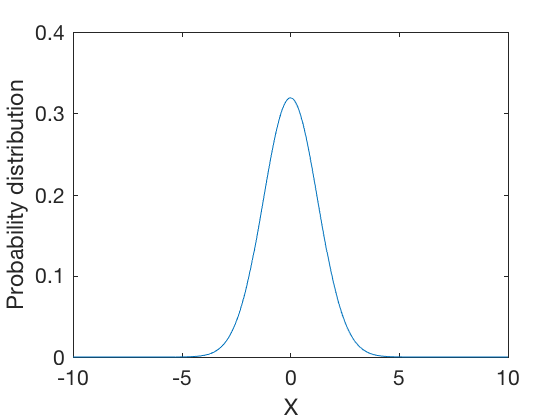
The normal distribution is represtented by a bell curve. The probability density function is represented as as

$f(X| \mu, \sigma^2) = \frac{1}{\sqrt{2 \pi \sigma^2}} e^{ - \frac{(X-\mu)^2}{2 \sigma^2}}$

where, $ \mu $ is the mean and $ \sigma $ is the standard deviation of the distribution.

clc
close all
clear all

X = -10:0.01:10;
mu = 0;
sigma = 1.25;
f_x = 1/sqrt(2*pi*sigma^2) * exp( -(X-mu).^2/(2*sigma^2) );
figure;
plot(X,f_x)
axis([-10 10 0 .4])
xlabel('X')
ylabel('Probability distribution')

Bayesian rule for Gaussian probabilities

We previously saw that the Bayesian estimates can be obtained by multiplying probability distributions. If we model the sensor noise and movement process as Gaussian distributions, we can compute probability of robot’s location using the techniques from before. However, this process involves computing multiplication of probability distributions.

Consider two normal probability distributions given by,

$f(X| \mu_1, \sigma_1^2) = \frac{1}{\sqrt{2 \pi \sigma_1^2}} e^{ - \frac{(X-\mu_1)^2}{2 \sigma_1^2}}$ $f(X| \mu_2, \sigma_2^2) = \frac{1}{\sqrt{2 \pi \sigma_2^2}} e^{ - \frac{(X-\mu_2)^2}{2 \sigma_2^2}}$

The Bayesian probability is given by,

$f((X| \mu_1, \sigma_1^2)|(X| \mu_2, \sigma_2^2)) = \frac{f(X| \mu_1, \sigma_1^2) f(X| \mu_2, \sigma_2^2)}{\int_{-\infty}^{\infty}f(X| \mu_1, \sigma_1^2) f(X| \mu_2, \sigma_2^2)dX}$

The product of two probability functions is given by,

$f((X| \mu_1, \sigma_1^2)|(X| \mu_2, \sigma_2^2)) = \frac{1}{\sqrt{2 \pi \sigma_1^2}} e^{ - \frac{(X-\mu_1)^2}{2 \sigma_1^2}}\frac{1}{\sqrt{2 \pi \sigma_2^2}} e^{ - \frac{(X-\mu_2)^2}{2 \sigma_2^2}}$ $f(X| \mu_1, \sigma_1^2) | f(X| \mu_2, \sigma_2^2) = \frac{1}{\sqrt{4 \pi^2 \sigma_1^2 \sigma_2^2}} e^{ - \left[ \frac{(X-\mu_1)^2}{2 \sigma_1^2} + \frac{(X-\mu_2)^2}{2 \sigma_2^2} \right]}$ $f(X| \mu_1, \sigma_1^2) | f(X| \mu_2, \sigma_2^2) = \frac{1}{\sqrt{4 \pi^2 \sigma_1^2 \sigma_2^2}} e^{ - \left[ \frac{ (\sigma_1^2+\sigma_2^2) X^2- 2 ( \mu_1 \sigma_2^2 + \mu_2 \sigma_1^2 ) X + (\mu_1^2 \sigma_2^2 + \mu_1^2 \sigma_1^2)}{2 \sigma_1^2 \sigma_2^2} \right]}$

After significant algebra, the final conditional probability, can be represented as,

$f(X| \mu_1, \sigma_1^2) | f(X| \mu_2, \sigma_2^2) = f(X| \mu_{12}, \sigma_{12}^2) = \frac{1}{\sqrt{2 \pi \sigma_{12}^2}} e^{ - \frac{(X-\mu_{12})^2}{2 \sigma_{12}^2}} ,$

where,

$\sigma_{12}^2 = \frac{\sigma_1^2 \sigma_2^2}{\sigma_1^2+\sigma_2^2}$

and

$\mu_{12} = \frac{\sigma_1^2 \mu_2 + \sigma_2^2 \mu_1}{\sigma_1^2+\sigma_2^2} .$

The expressions above show that the normalized convolution of two Gaussian distributions is a Gaussian distribution whose standard deviation is harmonic mean of the two distributions, and whose means is weighted by inverse of their variances. This results in a distribution where the mean gets skewed towards distribution with lower standard deviation. Further, the combined variance is inverse of the sum of inverses of variances of the two distributions. Therefore, the resulting variance is lower than variances of either distributions. In the special case when the variances of the original distributions are equal, the variance of the combined distribution is half the variance of either one. These are illustrated in examples below,

Gaussian Example 1: combined probability

$ \sigma_1 = .8 , \mu_1 = 2 $
$ \sigma_2 = .5 , \mu_2 = 4 $

$\sigma_{12}^2 = \frac{\sigma_1^2 \sigma_2^2}{\sigma_1^2+\sigma_2^2} = 3.2$

and

$\mu_{12} = \frac{\sigma_1^2 \mu_2 + \sigma_2^2 \mu_1}{\sigma_1^2+\sigma_2^2} = 0.66 .$

clc;close all;clear all

X = -10:0.01:10;
mu1 = .8 ; sigma1 = 2;
mu2 = .1 ; sigma2 = 4;

mu12 = (sigma1^2*mu2 + sigma2^2*mu1)/(sigma1^2 + sigma2^2);
sigma12 = sqrt((sigma1^2*sigma2^2)/(sigma1^2 + sigma2^2));

display(['\mu_{12} = ' num2str(mu12) ', \sigma_{12} = ' num2str(sigma12)] )

f1 = 1/sqrt(2*pi*sigma1^2) * exp( -(X-mu1).^2/(2*sigma1^2) );
f2 = 1/sqrt(2*pi*sigma2^2) * exp( -(X-mu2).^2/(2*sigma2^2) );
f12 = 1/sqrt(2*pi*sigma12^2) * exp( -(X-mu12).^2/(2*sigma12^2) );
figure;
plot(X,f12,X,f1,'g--',X,f2,'g--')
axis([-10 10 0 .4])
xlabel('X')
ylabel('Probability distribution')

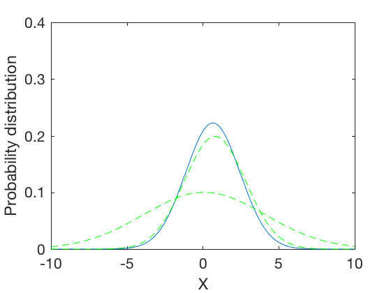
\mu_{12} = 0.66, \sigma_{12} = 1.7889

Gaussian Example 1: combined probability

$ \sigma_1 = -4 , \mu_1 = 4 $
$ \sigma_2 = 4 , \mu_2 = 4 $

$\sigma_{12}^2 = \frac{\sigma_1^2 \sigma_2^2}{\sigma_1^2+\sigma_2^2} = 2$

and

$\mu_{12} = \frac{\sigma_1^2 \mu_2 + \sigma_2^2 \mu_1}{\sigma_1^2+\sigma_2^2} = 0.$

clc;close all;clear all

X = -10:0.01:10;
mu1 = -4 ; sigma1 = 2;
mu2 = 4 ; sigma2 = 2;

mu12 = (sigma1^2*mu2 + sigma2^2*mu1)/(sigma1^2 + sigma2^2);
sigma12 = sqrt((sigma1^2*sigma2^2)/(sigma1^2 + sigma2^2));

display(['\mu_{12} = ' num2str(mu12) ', \sigma_{12} = ' num2str(sigma12)] )

f1 = 1/sqrt(2*pi*sigma1^2) * exp( -(X-mu1).^2/(2*sigma1^2) );
f2 = 1/sqrt(2*pi*sigma2^2) * exp( -(X-mu2).^2/(2*sigma2^2) );
f12 = 1/sqrt(2*pi*sigma12^2) * exp( -(X-mu12).^2/(2*sigma12^2) );
figure;
plot(X,f12,X,f1,'g--',X,f2,'g--')
axis([-10 10 0 .4])
xlabel('X')
ylabel('Probability distribution')

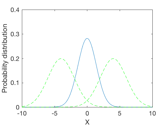
\mu_{12} = 0, \sigma_{12} = 1.4142

Gaussian 2-D distribution

The estimation techniques we developed so far apply only to 1-dimension systems, i.e. in cases where there is only 1 unknown variable. In cases where there are more than 1 unknown variable, we utilize multivariate distributions. The main idea of multivariate is illustrated in the figure below,

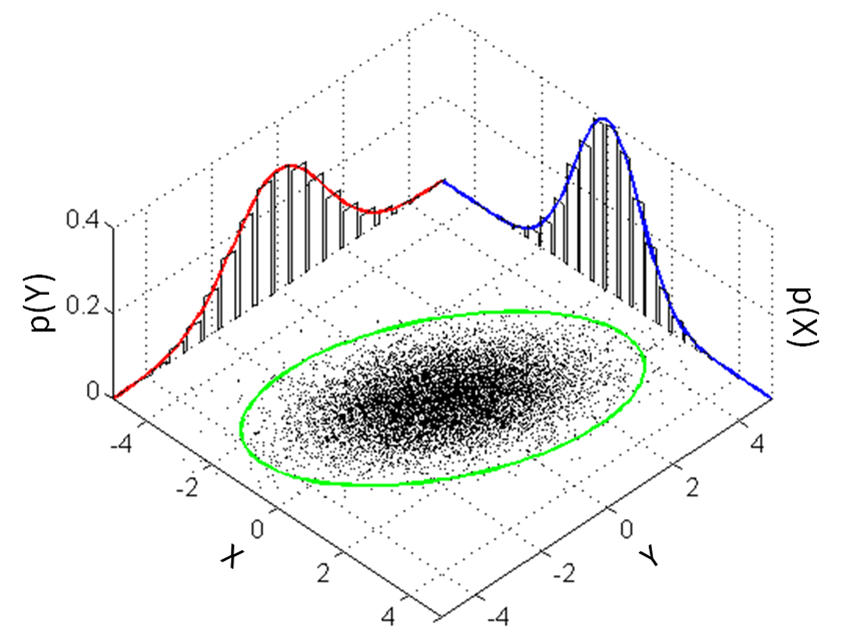
A multi-variate distribution of 2 variables is characterized by two univariate distributions where the center of multivariate distribution is the location of the means of other distribution. A multivariate distribution in $ k$ dimensions is represented as,

$f(X| \mathbf{\mu}, \mathbf{\Sigma}) = \frac{1}{\sqrt{ (2 \pi)^k |\mathbf{\Sigma}| }} e^{ - \frac{1}{2} (X-\mathbf{\mu})^T \mathbf{\Sigma}^{-1} (X-\mathbf{\mu}) }$

Where $ \Sigma $ is the covariance matrix, and $ \mu $ is the mean of the distribution. In the special case when $ K = 2 $, we have

$\mathbf{\Sigma} = \left[ \begin{array}{cc} \sigma_X^2 & \sigma_{X,Y} \\ \sigma_{X,Y} & \sigma_Y^2 \end{array} \right]$

where $ \sigma_{X,Y} $ is the second moment between x- and y- variables.

Kalman filter 2-D

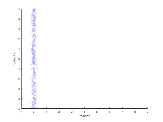
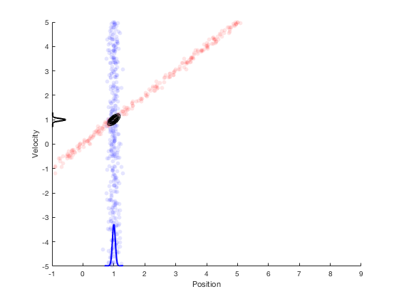
The techniques developed above combined with system dynamics information lead to Kalman filters. Kalman filters perform state estimation in two primary steps. The first step involves propogation of system dynamics to obtain apriori probability of states, once the measurements are obtained the state variables are updated using Bayesian theorm. This is illustrated by the example below. Consider the case of a car moving along a straight line with a fixed velocity. Further, say we have measurement on position only, and not velocity. At start, only the position is known from the sensor, so the region where the robot’s states could lie is shown in the figure below.

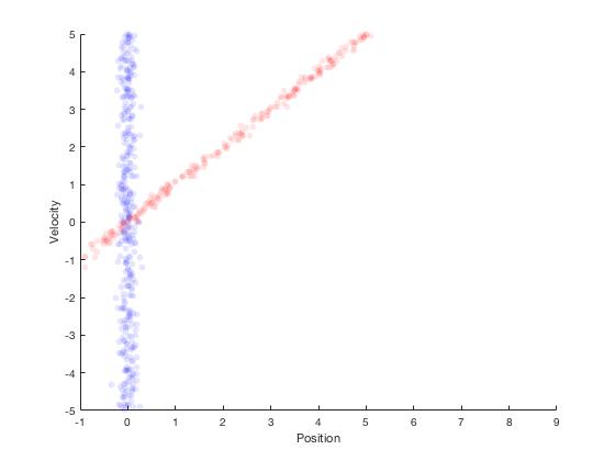
If the robot were to simply stay here, then its velocity could not be estimated. However, if the robot were to move, then the probability distribution after moving for 1 second with constant velocity is shown in red in the figure below.

Assuming that the robot moves with a velocity of 1, the next position estimate is around 1. By performing a second measurement at this point, we get the region in blue as the possible values of the position estimate.

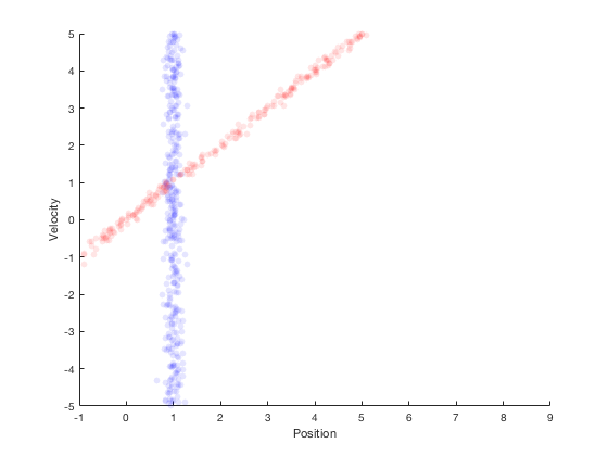
Therefore, from system dynamics, we expect the new position to be in the red region, and from sensors we expect the states to be in the blue region. The overlapping region between these two distributions is very small, and Bayes’ theorem can be applied to estimate the multivariate state distribution probability. The corresponding probability distributions of velocity and position are presented along x- and y- axis. This process of combining system dynamics with state measurements is the underlying principle of Kalman filters. Kalman filters provide good estimation properties and are optimal in the special case when the process and measurement follow a Gaussian distributions.

Kalman filters: optimality

In the previous section we saw how by combining information from system dynamics and sensors, a better estimate of states of the system can be obtained. We however, did not look into how to combine information from system dynamics and sensor measurement. To do so, we perform an optimization process where we maximize the likelihood of the states belonging to a region. This is also referred as maximum likelhood estimate.

Maximum likelihood estimator: Linear regression example

The likelyhood of a value coming from a given distribution is given by a probability desity function. Therefore, in the special case where the distribution is normal, the likelyhood of seeing a value $ X $ is given by,

$p(X| \mu, \sigma^2) = \frac{1}{\sqrt{2 \pi \sigma^2}} e^{ - \frac{(X-\mu)^2}{2 \sigma^2}}$

Say we have a specific task of determining pameters $ \beta_0$ and $ \beta_1 $ such that the likelihood of a given value $ y $ being of the form $ \beta_0 + \beta_1 X $ is maximized, i.e. the goal is to estimate parameters $ \beta_0$ and $ \beta_1 $ so the probability of error coming from a linear approximation in states is maximized. Further, we assume that the errors are distributed normally and have zero expected mean. In this case, the probability of seeing an error of $ e_i = y_i - (\beta_0+ \beta_1 x_i) $ becomes,

$p(e_i| 0, \sigma^2) = \frac{1}{\sqrt{2 \pi \sigma^2}} e^{ - \frac{(y_i - (\beta_0+ \beta_1 x_i))^2}{2 \sigma^2}}$

Therefore, the probability of seeing errors $ e_1, e_2, \dots , e_N $ becomes,

$p( e_1, e_2, \dots , e_N ) = \underbrace{\Pi}_{i=1~to~n} p(e_i| 0, \sigma^2)$

where $ \Pi $ stands for multiplication of probabilities.

$p( e_1, e_2, \dots , e_N ) = \underbrace{\Pi}_{i=1~to~n} p(e_i| 0, \sigma^2) = \underbrace{\Pi}_{i=1~to~n} \frac{1}{\sqrt{2 \pi \sigma^2}} e^{ - \frac{(y_i - (\beta_0+ \beta_1 x_i))^2}{2 \sigma^2}}$

Therefore, the goal of optimization routine is to find parameters to maximize the likelihood function. As the parameters $ \beta_0$ and $ \beta_1 $ appear only in the exponent, we can take log of the likelihood function.

$\underbrace{Maximize}_{\beta_0,\beta_1}~log(p( e_1, e_2, \dots , e_N )) = \underbrace{Maximize}_{\beta_0,\beta_1}\sum_{i=1}^N \left(- \frac{(y_i - (\beta_0+ \beta_1 x_i))^2}{2 \sigma^2} - \frac{1}{2}log(2 \pi \sigma^2) \right)$

The expression above is also called maximum log likelihood. As we are maximizing the negative of a value, and as we are addining and multiplying by constants, the maximizing likelihood problem can be rewritten as,

$\underbrace{Minimize}_{\beta_0,\beta_1}\sum_{i=1}^N \left(y_i - (\beta_0+ \beta_1 x_i) \right)^2,$

i.e. in this case, the maximum likelihood function reduces to finding the least-square fit line. A similar process can be applied to compute the state estimates in kalman filter.

Particle filters

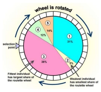
Particle filters are a class of simulation-based filter, unlike model-based. In this case, we do not assume anything about the underlying model of the plant. The primary idea is to sample the space for all possible values of states, and assign weights to each point depending on how close it is to the measurement from the actual plant. Once the weights are obtained, the plant’s states are resampled with probability of survival of each particle being proportional to its weight. Over time, the points whose measurements correspond to highly unlikely states vanish, and points that are more likely are retained. The weight is typically chosen as multi-variate gaussian distribution. The resampling is best illustrated by a roulette wheel selection, where each particle’s chance of survival is determined based on how large an area it occupies on the wheel.

Animation below presents implementation of particle-filter for a simple 2D SLAM for cases where sensor noise is high and low.