Kalman filter

Vivek Yadav, PhD

We previously reviewed concepts of probability, and saw how by repeatedly measuring and moving a robot could estimate its velocity and position. We will now extend these ideas to formally describe Kalman filters. Kalman filters are observer equivalent of linear quadratic regulators and are also called linear quadratic estimators.

Discrete kalman filter.

As estimation via kalman filtering involves successively measurement and state propogation, they are easier to understand via discrete implementation. Consider a system given by,

$X_{k+1} = AX_{k} + Bu_{k} + Fw_{k}$

where $ w_k $ is uncertainity in the system dynamics that is represented as a Gaussian process, with covariance $ E(w_k w_k^T ) = Q $. The state variables $ X_k $ are also modeled as mutually independent Gaussian processes with covariance $ P_k $. The initial conditions are now given as, $X(0) = X_0 $ and covariance $ P_0 $.

Measurement is approximated as,

$Y_k = CX_k + Du_k + v_k$

where $ v_k $ is uncertainity in the measurement with covariance $ E(v_k v_k^T ) = R $.

As with previous Kalman 2D example, we will perform the process of measurement and state propogation successively.

1. State propogation

System dynamics are given by,

$X_{k+1} = AX_{k} + Bu_{k} + F w_{k}$

To separate the state estimates before and after measurement, we define,

$ X_{k k} $ as estimate after measurement at step k.
$ X_{k+1 k} $ is the state estimate after following system dynamics.

Therefore the expected future value of the state are given by,

$E(X_{k+1|k} ) = AE(X_{k|k} ) + BE(u_k) + E(F w_k)$ $\hat{X}_{k+1|k} = A\hat{X}_{k|k} + B u_k$

The error between state estimate and expected value, before getting measurement is represented as,

$X_{k+1|k} - \hat{X}_{k+1|k} = AX_{k|k} + Bu_k + F w_k -( A\bar{X}_{k|k} + Bu_k )$ $e_{k+1|k} = X_{k+1|k} - \bar{X}_{k+1|k} = Ae_{k|k} + F w_k$

Therefore, the covariance of state before getting measurement is given by,

$P_{k+1|k} = E(e_{k+1|k} e_{k+1|k}^{-T}) = P( (X_{k+1|k}- \bar{X}_{k+1|k})(X_{k+1|k} - \bar{X}_{k+1|k})^T)$ $P_{k+1|k} = A E(e_{k|k} e_{k|k}^T) A^T + E(Fw_k w_k^TF^T)$

Therefore, the error covariance propogation is given by,

$P_{k+1|k} = A P_{k|k} A^T + FQF^T .$

2. Update

We now update covariance of state estimates after getting the measurement. The measurement are given by,

$Y_{k+1} = CX_{k+1|k} + Du_{k+1} + v_{k+1}$

The expected value of measurement is given by,
$\hat{Y}_{k+1} = C \hat{X}_{k+1|k}+ Du_{k+1} .$

The error between state estimate and mean is given by,

$Y_{k+1} - \hat{Y}_{k+1}= CX_{k+1|k} + Du_{k+1} + v_{k+1} - ( C \hat{X}_{k+1|k} + Du_{k+1})$ $e_{Y,k+1} = Ce_{k+1|k} + v_{k+1}$

The covariance of measurement error before getting measurement is given by,

$E(e_{Y,k+1} e_{Y,k+1}^T) = E((Ce_{k+1|k} + v_{k+1})(Ce_{k+1|k} + v_{k+1})^T)$ $E(e_{Y,k+1} e_{Y,k+1}^T) = E((Ce_{k+1|k} + v_{k+1})(e_{k+1|k}^TC^T + v_{k+1}^T))$ $= CP_{k+1|k}C^T + R$

State update after measurement

State update after measurement is given by,

$\hat{X}_{k+1|k+1} = \hat{X}_{k+1|k}+ K_{k+1}(Y_{k+1} - ( C \hat{X}_{k+1|k} + Du_{k+1}) )$ $\hat{X}_{k+1|k+1} = \hat{X}_{k+1|k} + K_{k+1}e_{Y,k+1}$ $\hat{X}_{k+1|k+1} = \hat{X}_{k+1|k} + K_{k+1}C e_{k+1|k} +K_{k+1}v_{k+1}$

i.e. the state estimate is updated based on error between the actual measurement and expected measurement from state estimate. Objective is to find $ K_{k+1}) $ such that the difference between actual and estimated state is minimum.

The objective is to choose a gain so the error between posterior state estimate and actual state is minimum.

$X_{k+1}- \hat{X}_{k+1|k+1} = X_{k+1}- \hat{X}_{k+1|k} - K_{k+1}C e_{k+1|k} -K_{k+1}v_{k+1}$ $e_{k+1|k+1} = (I - K_{k+1}C) e_{k+1|k} - K_{k+1} v_{k+1}$

Therefore, the posterior covariance becomes

$P_{k+1|k+1} = E( e_{k+1|k+1} e_{k+1|k+1}^T )$ $= E \left( ( (I - K_{k+1}C) e_{k+1|k} - K_{k+1} v_{k+1} ) ( (I - K_{k+1}C) e_{k+1|k} - K_{k+1}v_{k+1} ) ^T \right)$ $= (I - K_{k+1}C) E (e_{k+1|k} e_{k+1|k}^T) (I - K_{k+1}C)^T + K_{k+1} E(v_{k+1} v_{k+1}^T) K_{k+1}^T$ $P_{k+1|k+1} = (I - K_{k+1}C) P_{k+1|k} (I - K_{k+1}C)^T + K_{k+1}R K_{k+1}^T$ $P_{k+1|k+1} = (I - K_{k+1}C) P_{k+1|k} (I - K_{k+1}C)^T + K_{k+1} R K_{k+1}^T$ $P_{k+1|k+1} = P_{k+1|k} - K_{k+1}C P_{k+1|k} - P_{k+1|k} C^T K_{k+1}^T + K_{k+1} (C P_{k+1|k} C^T + R) K_{k+1}^T$

As the trace of covariance matrix is the error between state estimate and update from measurement, therefore, the gain matrix that minimizes the covariance matrix is the optimal solution. Taking derivative with respect to gain gives,

$\frac{\partial tr(P_{k+1|k+1} )}{\partial K_{k+1} } = -2 (CP_{k+1|k})^T + 2K_{k+1} (C P_{k+1|k} C^T + R) = 0$

Therefore,

$K_{k+1} = P_{k+1|k}C^T(C P_{k+1|k} C^T + R)^{-1}$

Substituting $ K_{k+1} $ in expression for posterior covariance gives,

$P_{k+1|k+1} = P_{k+1|k} - K_{k+1}C P_{k+1|k} - K_{k+1}C^T P_{k+1|k}^T + P_{k+1|k}C^T(C P_{k+1|k} C^T + R)^{-1}(C P_{k+1|k} C^T + R) K_{k+1}^T$ $P_{k+1|k+1} = P_{k+1|k} - K_{k+1}C P_{k+1|k} - K_{k+1}C^T P_{k+1|k}^T + P_{k+1|k}C^TK_{k+1}^T$ $P_{k+1|k+1} = P_{k+1|k} - K_{k+1}C P_{k+1|k} = ( I - K_{k+1}C ) P_{k+1|k}$

Final form of Kalman filter

1. State propogation

$\hat{X}_{k+1|k} = A\hat{X}_{k|k} + Bu_k$ $P_{k+1|k} = A P_{k|k} A^T + FQF^T .$

2. Measurement update

$e_{Y,k+1} = y(k+1) - ( C \hat{X}_{k+1|k} + Du_{k+1})$ $S_{k+1} = (C P_{k+1|k} C^T + R)$ $K_{k+1} = P_{k+1|k} C^TS_{k+1}^{-1}$ $\hat{X}_{k+1|k+1} = \hat{X}_{k+1|k} + K_{k+1}e_{Y,k+1}$ $P_{k+1|k+1} = ( I - K_{k+1}C ) P_{k+1|k}$

Kalman filter: Example 1

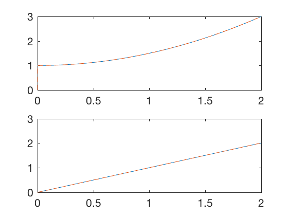
We first apply kalman filter to estimate states in the simplest case where we have a deterministic process and measurement. Consider the system give

$\ddot{X} = u$

with measurement $ y = X $. We wish to develop an observer such that the states of the observer $ \hat{X} \rightarrow X $.

We approximate this system as follows,

$X_1(t+1) = X_1(t) + \delta t X_2$ $X_2(t+1) = \delta t u$

The measurement is approximated as

$y = X + v$

where $ v $ is a Gaussian process with mean 0, and variance $ 10^{-8} $. Note as the system is determinitistic, we use a very low value of measurement covariance $ R $. The MATLAB code below implements Kalman filter for state estimation. As we do not know the covariance of states apriori, we assume it to start as identity matrix. The states are estimated in 1 iteration, and the error goes to zero very fast.

clc
close all
clear all


A = [0 1 ; 0 0];
B = [0 ; 1];
dt = 0.001;

Ad = eye(2) + dt*[0 1 ; 0 0];
Bd = dt*B;

C = [1 0];
R = 1e-8;
Q = 0*eye(2);
P_pl = eye(2);
X_hat_0 = [0;0];

X_0 = [1;0];

X(:,1)= X_0;
Y(1) = C*X(:,1);
t(1) = 0;
X_hat(:,1)= X_hat_0;

for i = 1:2000
    u = 1;
    
    t(i+1) = t(i)+dt;
    
    % True process 
    X(:,i+1)=Ad * X(:,i) + Bd*u;
    Y(i+1) = C*X(:,i+1);
    
    P_mi = Ad*P_pl*Ad' + Q;
    X_hat(:,i+1)=Ad * X_hat(:,i) + Bd*u;
    
    
    Y_hat(i+1) = C*X_hat(:,i+1);
    
    
    e_Y  = Y(i+1) - Y_hat(i+1);
    S = C*P_mi*C'+R;
    K = P_mi*C'*inv(S);
    P_pl = (eye(2) - K*C)*P_mi;
    X_hat(:,i+1)=X_hat(:,i+1) + K*e_Y;
end

figure;
subplot(2,1,1)
plot(t,X(1,:),t,X_hat(1,:),'--')
subplot(2,1,2)
plot(t,X(2,:),t,X_hat(2,:),'--')

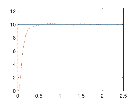
Kalman filter for parameter estimation: Example 2 (position measurement only)

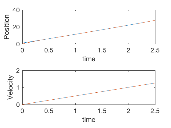
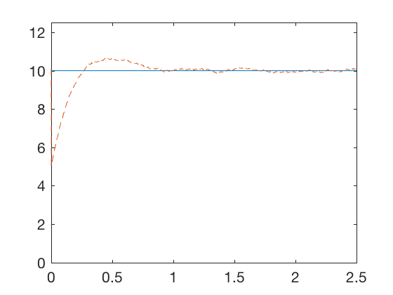
Kalman filters can be used for parameter estimation also. Consider the dynamic system given by,

$\dot{X_1} = X_2 + \alpha$ $\dot{X_2} = u$

where $ \alpha $ is a parameter that is unknown. The only measurement $ y = X_1 + v$ is available, where $ v $ is a Gaussian process with variance $ R = .1 $. We can apply Kalman filtering technique for estimating the unknown parameter. We add a new state to system, which is the parameter itself. And introduce the dyamics that the derivative is zero. As we do not know the parameter accurately, we introduce a noise term in the system dynamics to account for uncertainity in the model.

$X_1(t+1) = X_1(t) + \delta t X_2 + \delta t X_3$ $X_2(t+1) = \delta t u$ $X_3(t+1) = X_3(t) + w(t)$

where $ w(t) $ is a Gaussian process with covariance $ 10^{-4} $. The expression above can be written in the form of

$X_{t+1} = AX_{t} + Bu_{t} + Fw_t$ ,

where

$A = \left[ \begin{array}{ccc} 1 & \delta t & \delta t \\ 0 & 0 & 0 \\ 0 & 0 & 0\end{array} \right]$ $B = \left[ \begin{array}{c} 0 \\ \delta t \\ 0\end{array} \right]$ $F = \left[ \begin{array}{c} 0 \\ 0 \\ 1\end{array} \right]$

At start, we do not know the state covariance, so we approximate it as 1. However, accurate covairance measure is required to estimate the state. Therefore, we run simulation (or conduct experiment) once to estimate the covariance and start and repeat the process again. Repeating this proces multiple times (typically 2) gives a close enough estimate of the unknown parameter.

clc
close all
clear all


A = [0 1 1; 0 0 0;0 0 0];
B = [0 ; 1;0];

dt = 0.001;

Ad = eye(3) + dt*A;
Bd = dt*B;
F = [0;0;1];

C = [1 0 0];
R = .1;
Q = diag([1e-4]);
P_pl = eye(3);

X_hat_0 = [0;0;0];
X_0 = [1;0;10];

X(:,1)= X_0;
Y(:,1) = C*X(:,1);
t(1) = 0;
X_hat(:,1)= X_hat_0;

for i_sim = 1:2
    A_sim(i_sim) = X_hat(3,1);
    for i = 1:2500
        u = .5;
        
        t(i+1) = t(i)+dt;
        
        % True process
        X(:,i+1)=Ad * X(:,i) + Bd*u;
        Y(:,i+1) = C*X(:,i+1) + sqrt(R)*randn(1,1);
        
        % Observer model
        % Prediction based on system dynamics
        P_mi = Ad*P_pl*Ad' + F*Q*F';
        X_hat(:,i+1)=Ad * X_hat(:,i) + Bd*u;
        Y_hat(:,i+1) = C*X_hat(:,i+1);
        
        % Update based on measurement
        e_Y  = Y(:,i+1) - Y_hat(:,i+1);
        S = C*P_mi*C'+R;
        K = P_mi*C'*inv(S);
        P_pl = (eye(3) - K*C)*P_mi;
        X_hat(:,i+1)=X_hat(:,i+1) + K*e_Y;
    end
    X_hat(3,1) = X_hat(3,end);
    
end

figure;
subplot(2,1,1)
plot(t,X(1,:),t,X_hat(1,:),'--')
axis([0 2.5 0 40])
xlabel('time')
ylabel('Position')

subplot(2,1,2)
plot(t,X(2,:),t,X_hat(2,:),'--')
xlabel('time')
ylabel('Velocity')
axis([0 2.5 0 2])

figure;
plot(t,X(3,:),t,X_hat(3,:),'--')
axis([0 2.5 0 12.5])

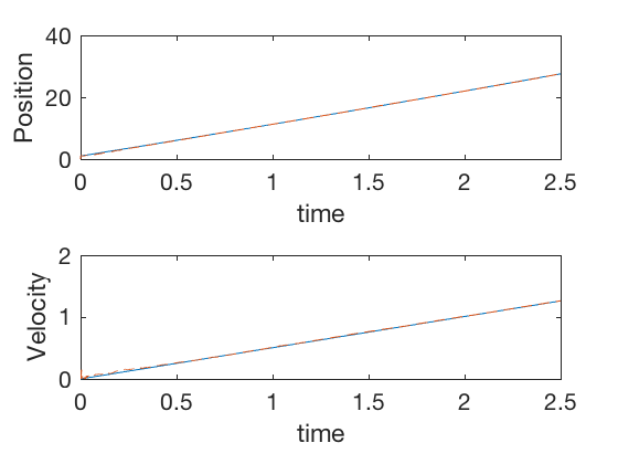
Kalman filter for parameter estimation: Example 3 (position and velocity measurement)

Kalman filters can be used for parameter estimation also. Consider the dynamic system given by,

$\dot{X_1} = X_2 + \alpha$ $\dot{X_2} = u$

where $ \alpha $ is a parameter that is unknown. The measurements $ y_1 = X_1 + v_1$ and $ y_2 = X_2 + v_2$ are available, where $ v $s are Gaussian processes with variances $ R_1 = .1 , R_2 = .1 $. We can apply Kalman filtering technique for estimating the unknown parameter.

$X_1(t+1) = X_1(t) + \delta t X_2 + \delta t X_3$ $X_2(t+1) = \delta t u$ $X_3(t+1) = X_3(t) + w(t)$

where $ w(t) $ is a Gaussian process with covariance $ 10^{-4} $. As before, we run simulation (or conduct experiment) once to estimate the covariance and start and repeat the process again. Repeating this proces multiple times (typically 2) gives a close enough estimate of the unknown parameter.

clc
close all
clear all


A = [0 1 1; 0 0 0;0 0 0];
B = [0 ; 1;0];
dt = 0.001;

Ad = eye(3) + dt*A;
Bd = dt*B;


F = [0;0;1];

C = [1 0 0;
     0 1 0];
R = diag([.1 .1]);
Q = diag([1e-4]);
P_pl = eye(3);

X_hat_0 = [0;0;0];
X_0 = [1;0;10];

X(:,1)= X_0;
Y(:,1) = C*X(:,1);
t(1) = 0;
X_hat(:,1)= X_hat_0;

for i_sim = 1:1
    A_sim(i_sim) = X_hat(3,1);
    for i = 1:2500
        u = .5;
        
        t(i+1) = t(i)+dt;
        
        % True process
        X(:,i+1)=Ad * X(:,i) + Bd*u;
        Y(:,i+1) = C*X(:,i+1) + sqrt(R)*randn(2,1);
        
        
        % Observer model
        % Prediction based on system dynamics
        P_mi = Ad*P_pl*Ad' + F*Q*F';
        X_hat(:,i+1)=Ad * X_hat(:,i) + Bd*u;
        Y_hat(:,i+1) = C*X_hat(:,i+1);
        
        % Update based on measurement
        e_Y  = Y(:,i+1) - Y_hat(:,i+1);
        S = C*P_mi*C'+R;
        K = P_mi*C'*inv(S);
        P_pl = (eye(3) - K*C)*P_mi;
        X_hat(:,i+1)=X_hat(:,i+1) + K*e_Y;
    end
    X_hat(3,1) = X_hat(3,end);
    
end

figure;
subplot(2,1,1)
plot(t,X(1,:),t,X_hat(1,:),'--')
axis([0 2.5 0 40])
xlabel('time')
ylabel('Position')

subplot(2,1,2)
plot(t,X(2,:),t,X_hat(2,:),'--')
xlabel('time')
ylabel('Velocity')
axis([0 2.5 0 2])

figure;
plot(t,X(3,:),t,X_hat(3,:),'--')
axis([0 2.5 0 12.5])

Kalman filter: Continuous system (Kalman-Bucy filter)

Kalman-Bucy filter is continuous time equivalent of Kalman filter. Kalman filter is difficult to derive and interpret for continuous systems because the measurement and states both are continuous variables, and the apriori and posteriori updates are not clearly defined. However, by discretizing the continuous filter, and taking limit as the discretization time goes to zero gives equations for kalman filter. Detailed derivation can be found here.

Consider the system dynamics given by,

$\dot{X} = AX + Bu + Fw$

where $ w $ is a Gaussian process with zero mean and covariance $ Q $, and measurement given by

$y = CX + Du + v$

The filter for state estimate consists of 2 differential equations,

$\dot{\hat{X}} = A \hat{X} + Bu + K ( y - C \hat{X}+ Du)$ $\dot{P} = A P + PA^T + FQF^T - K R K^T$ $K = P C^T R^{-1}$ $\dot{P} = A P + PA^T + FQF^T - P C^T R CP$

Note, in continuous case, the measurement error’s covariance and apriori covairance both are $ R $. Further, the observer gain calculations involve taking inverse of the covariance of noise $ R $ matrix. Therefore, if we had 2 sensors, one very noisy and other very accurate, the kalman filter will place more value on the accurate sensor, i.e. the sensor with lower covariance noise will contribute more to the update. Note, the equation above is analogous to the Riccati equation we saw while deriving conditions for linear quadratic regulator, and can be solved using similar technique. In the special infitite-time case, the riccati equation becomes,

$0 = A P + PA^T + FQF^T - P C^T R CP$

The equation above is the same as infitite time algebraic Riccati equation with A and B replaced by $A^T $ and $C^T$, and can be solved using care command in MATLAB.

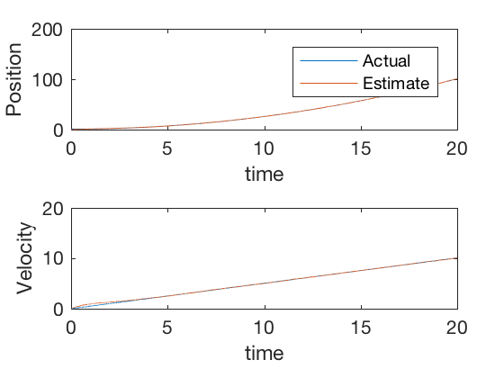
Kalman filter continuous time: Example 1

Consider the system given by, $ \ddot{x} = u $, with measurement on position alone. We will fit a continuous time kalman filter to the model by assuming a unity covarance for measurement noise and identity for process covariance. MATLAB’s care command was used to solve the algebraic Riccati equation.

clc
close all
clear all


A = [0 1;0 0];
B = [0; 1];
C = [1 0];

t = 0:0.001:20; 
dt = t(2) - t(1);
X(:,1) = [1;0];
y(:,1) = C*X;
R_k = diag([1 ]);
Q_k = diag([1 1]);
P_k = care(A',C',Q_k,R_k);
K_k = P_k*C'*inv(R_k);
L = K_k;

X_hat(:,1) = [0;0];
y_hat(:,1) = C*X_hat;
for i = 2:length(t)
    u = .5;
    
    X(:,i) = X(:,i-1)  +dt * (A*X(:,i-1) + B*u);
    y(:,i) = C*X(:,i) + sqrt(R_k)*randn(size(C,1),1);

    X_hat(:,i) = X_hat(:,i-1)  +dt * (A*X_hat(:,i-1) + B*u +L *(y(:,i-1)-y_hat(:,i-1)));
    y_hat(:,i) = C*X_hat(:,i) ;
end


figure;
subplot(2,1,1)
plot(t,X(1,:),t,X_hat(1,:))
legend('Actual','Estimate')
xlabel('time')
ylabel('Position')
subplot(2,1,2)
plot(t,X(2,:),t,X_hat(2,:))
xlabel('time')
ylabel('Velocity')

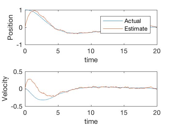
Kalman filter continuous time: Example 2 (two sensors)

Consider the same system as before that is given by, $ \ddot{x} = u $, with measurement on position alone. However, now we have 2 sensors to measure position, one sensor is very accurate (covariance = 0.01), while the other is not accurate (covariance = 1). We will fit a continuous time kalman filter to the model by assuming a identity for process covariance. MATLAB’s care command was used to solve the algebraic Riccati equation. The gains computed from infitite time steady state Riccati equation are,

$K_k = \left[ \begin{array}{cc} 0.1090 & 10.8956 \\ 0.0995 & 9.9504 \end{array} \right]$

The gain matrix from kalman filter places more importance on the data coming from the second more accurate sensor, and less on the noisy sensor.

clc
close all
clear all


A = [0 1;0 0];
B = [0; 1];
C = [1 0;
    1 0];

t = 0:0.001:20; 
dt = t(2) - t(1);
X(:,1) = [1;0];
y(:,1) = C*X;
R_k = diag([1 .01]);
Q_k = diag([1 1]);
P_k = care(A',C',Q_k,R_k);
K_k = P_k*C'*inv(R_k);
L = K_k;
K_k
X_hat(:,1) = [0;0];
y_hat(:,1) = C*X_hat;
for i = 2:length(t)
    u = .5;
    
    X(:,i) = X(:,i-1)  +dt * (A*X(:,i-1) + B*u);
    y(:,i) = C*X(:,i) + sqrt(R_k)*randn(size(C,1),1);

    X_hat(:,i) = X_hat(:,i-1)  +dt * (A*X_hat(:,i-1) + B*u +L *(y(:,i-1)-y_hat(:,i-1)));
    y_hat(:,i) = C*X_hat(:,i) ;
end


figure;
subplot(2,1,1)
plot(t,X(1,:),t,X_hat(1,:))
legend('Actual','Estimate')
xlabel('time')
ylabel('Position')
subplot(2,1,2)
plot(t,X(2,:),t,X_hat(2,:))
xlabel('time')
ylabel('Velocity')

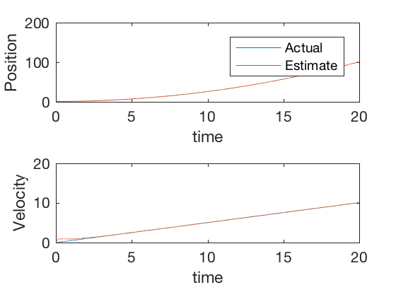
Linear Quadratic Gaussian

Linear Quadratic Gaussian control is a control scheme that uses Linear Quadratic Regulator (LQR) for control and kalman filter for estimation. From separation principle, we can design observer and controller separately without affecting performance of one or other. The script below implements a Linear Quadratic Regulator for control and continuous time Kalman filter using MATLAB’s care command.

clc
close all
clear all


A = [0 1;0 0];
B = [0; 1];
C = [1 0];

% Controller design
R = diag([1]);
Q = diag([1e-2 1e-2]);
M_a = rank(ctrb(A,B));
P = care(A,B,Q,R);
K_u  = inv(R)*B'*P;

t = 0:0.001:20; 
dt = t(2) - t(1);
X(:,1) = [1;0];
y(:,1) = C*X;

% Observer design
R_k = diag([1 ]);
Q_k = diag([1 1]);
P_k = care(A',C',Q_k,R_k);
K_k = P_k*C'*inv(R_k);
L = K_k;

X_hat(:,1) = [0;0];
y_hat(:,1) = C*X_hat;
for i = 2:length(t)
    u = -K_u*X_hat(:,i-1);
    
    X(:,i) = X(:,i-1)  +dt * (A*X(:,i-1) + B*u);
    y(:,i) = C*X(:,i) + sqrt(R_k)*randn(size(C,1),1);

    X_hat(:,i) = X_hat(:,i-1)  +dt * (A*X_hat(:,i-1) + B*u +L *(y(:,i-1)-y_hat(:,i-1)));
    y_hat(:,i) = C*X_hat(:,i) ;
end


figure;
subplot(2,1,1)
plot(t,X(1,:),t,X_hat(1,:))
legend('Actual','Estimate')
xlabel('time')
ylabel('Position')
subplot(2,1,2)
plot(t,X(2,:),t,X_hat(2,:))
xlabel('time')
ylabel('Velocity')

Conclusions

Kalman filters have been used extensively for several control and signal processing applications. Kalman filters are observer analogs of linear quadratic regulators, and can be derived using the same expressions by replacing system matrix by its transpose, and input matrix by transpose of measurement matrix. Kalman filters are optimal when the involved processes and measurements follow a Gaussian distribution. Kalman filters have been extended for nonlinear systems also, we will discuss these in coming classes.