Applying principles of linear control systems for control of nonlinear system dynamics

Vivek Yadav, PhD

Control design for nonlinear systems is a complete field in itself, which we will dive into in the coming classes. However many techniques developed for linear systems can be adopted for control of nonlinear systems. The main idea is to first compute a desired trajectory or a desired set point, linearize about this set point and apply linear control techniques for control.

Motivation

It is difficult to compute optimal control policies for most nonlinear systems. However, within a given neighborhood of states and control, the system behaves like a linear system. Therefore, if we compute a base trajecotry that roughly follows the dynamics of the system and gives optimal control under some simplified assumptions, we can construct a trajectory following controller by linearing the system about the desired trajectory and using techniques from linear control to drive errors to zero. The additional linearized control is also necessary to compensate for any unexpected perturbations that may be present due to external factors not accounted for in the controller design.

Control synthesis: General case

Consider the system given by,

$\dot{X} = f(X,u)$

where $ f$ represent the nonlinear functions that describe the equations of motion. Say using some trajectory planning algrithm like GPOPS II, we come up with a desired trajectory $ X_d $ that satisfies

$\dot{X_d} = f(X_d, u_d)$

where $d $ denotes the label corresponding for the desired trajectory, typically computed from some trajectory optimization algorithm. Taking error between the true and desired system dyanmic equations gives,

$\dot{X} - \dot{X_d} = f(X,u) - f(X_d,u_d)$

Defining $ e = X - X_d $ and $ \delta u = u - u_d $ , gives

$\dot{e} = f(X_d+e,u_d+\delta u) - f(X_d,u_d)$

Taking Taylor series expansion about $X_d$ gives,

$\dot{e} = f(X_d,u_d) + \left. \frac{\partial f}{ \partial X} \right|_{X_d,u_d} e + \left. \frac{\partial f}{ \partial u} \right|_{X_d,u_d} \delta u - f(X_d,u_d) + H.O.T$

Where HOT stands for higher order terms. Ignoring the higher order terms gives,

$\dot{e} = \left. \frac{\partial f}{ \partial X} \right|_{X_d,u_d} e + \left. \frac{\partial f}{ \partial u} \right|_{X_d,u_d} \delta u$

The expression above can be written as,

$\dot{e} = A_d e + B_d \delta u$

where,

$A_d = \left. \frac{\partial f}{ \partial X} \right|_{X_d,u_d}$ $B_d = \left. \frac{\partial f}{ \partial u} \right|_{X_d,u_d}$

All the techniques of linear control system can be applied to the system described above. Note the expression above depends on both the desired state and control varaibles. Note the final control to be applied to the system is given by,

$u = u_d + \delta u$

Stabilization

Stabilization is a special case of tracking where the desired trajectory is a fixed point, and the desired control is a fixed value (typically both are 0). The same control scheme developed above can be applied for stabilization too.

State dependent Riccati equation (SDRE)

SDRE control is a special case which results in systems that have valid linear-like approximation over a wide range, and can be expressed as $\dot{X} = A(X)X + B(X) u$

In the expression above, a linear quadratic controller can be designed assuming the state transition matrix $A(X)$ and input matrix $B(X)$ is constant at each time step, and using a Linear Quadratic Regulator to drive errors to zero. This results in a Riccati equation that depends on the current state value that needs to be solved at each time step along the trajectory. This technique is called SDRE control. A detailed example of SDRE control can be found here.

Control synthesis for robotic applications

Equations of motion of robots have many nice properties that can be exploited for design of controllers. We previously derived equations of motion of a robot as,

$M (q) \ddot{q} + C(q,\dot{q}) \dot{q} + G(q) = \tau$

As $ M(q) $ for robots is always invertible and positive definite, we get some nice properties that can be exploited for controller design. The acceleration relation for joint angles can be written as

$\ddot{q} = M(q)^{-1}ff(q,\dot{q},\tau).$

The expression above can be linearized about a desired trajectory as,

$\ddot{\delta q} = \ddot{q} - \ddot{q}_d \approx \left. \frac{\partial M(q)^{-1} ff}{ \partial q} \right|_{(q_d,\dot{q_d},\tau_d)} \delta q + M(q_d)^{-1} \left. \frac{\partial ff}{ \partial \dot{q}} \right|_{(q_d,\dot{q_d},\tau_d)} \delta \dot{q}+ M(q_d)^{-1} \left. \frac{\partial ff}{ \partial \tau} \right|_{(q_d,\dot{q_d},\tau_d)} \delta \tau$ $\ddot{\delta q} = \left( \left. \frac{\partial M(q)^{-1} }{ \partial q} \right|_{(q_d,\dot{q_d},\tau_d)} \circ ff \right) \delta q + M(q_d)^{-1}\left. \frac{\partial ff}{ \partial q} \right|_{(q_d,\dot{q_d},\tau_d)} \delta q + M(q_d)^{-1} \left. \frac{\partial ff}{ \partial \dot{q}} \right|_{(q_d,\dot{q_d},\tau_d)} \delta \dot{q}+ M(q_d)^{-1} \left. \frac{\partial ff}{ \partial \tau} \right|_{(q_d,\dot{q_d},\tau_d)} \delta \tau$

where,

$\left( \left. \frac{\partial M(q)^{-1} }{ \partial q} \right|_{(q_d,\dot{q_d},\tau_d)} \circ ff \right)$

is a tensor product between derivative of inverse of $ M(q) $ and $ ff $. The derivative of the inverse of mass matrix can be computed as,

$\frac{\partial M(q)^{-1} }{ \partial q} = - M(q)^{-1} \frac{\partial M(q)}{\partial q} M(q)^{-1}$

and

$ff(q,\dot{q},\tau) = (\tau - C(q,\dot{q}) \dot{q} - G(q)),$

Therefore, we can express the simplified linear system in state space form using the following variable transformations,

$\dot{\delta q}_1 = \delta q_2$ $\dot{\delta q}_2 \approx \left. \frac{\partial M(q)^{-1} ff}{ \partial q} \right|_{(q_d,\dot{q_d},\tau_d)} \delta q_1 + M(q_d)^{-1} \left. \frac{\partial ff}{ \partial \dot{q}} \right|_{(q_d,\dot{q_d},\tau_d)} \delta q_2+ M(q_d)^{-1} \left. \frac{\partial ff}{ \partial \tau} \right|_{(q_d,\dot{q_d},\tau_d)} \delta \tau$ $\frac{d}{dt} \left[ \begin{array}{c} \delta q_1 \\ \delta q_2 \end{array} \right] = \left[ \begin{array}{cc} 0 & I\\ \left. \frac{\partial M(q)^{-1} ff}{ \partial q} \right|_{(q_d,\dot{q_d},\tau_d)} & M(q_d)^{-1} \left. \frac{\partial ff}{ \partial \dot{q}} \right|_{(q_d,\dot{q_d},\tau_d)} \end{array} \right] \left[ \begin{array}{c} \delta q_1 \\ \delta q_2 \end{array} \right] + \left[ \begin{array}{c} 0 \\ M(q_d)^{-1} \left. \frac{\partial ff}{ \partial \tau} \right|_{(q_d,\dot{q_d},\tau_d)} \end{array} \right] \tau$

The expression above is a linear approximation of the system dynamics, and this approximation can be used to design controller for the true nonlinear system. For now, we will apply a high-gain controller to compensate for any errors introduced due to this linear approximation. However, the stability of the controller is not always guaranteed. In the coming classes, we will go over specifically how to analyze nonlinear controllers and test their stability.

** Note: Linearized matrices above can be computed and saved in file for calculations later, however in most cases, it is not possible to compute these matrices in symbolic form directly. Especially in cases wehre the number of states is very high. So the easier to compute matrices are calculated and saved as function, and the linearized matrices are calculated on the fly according with the equation below. **

MATLAB Demo

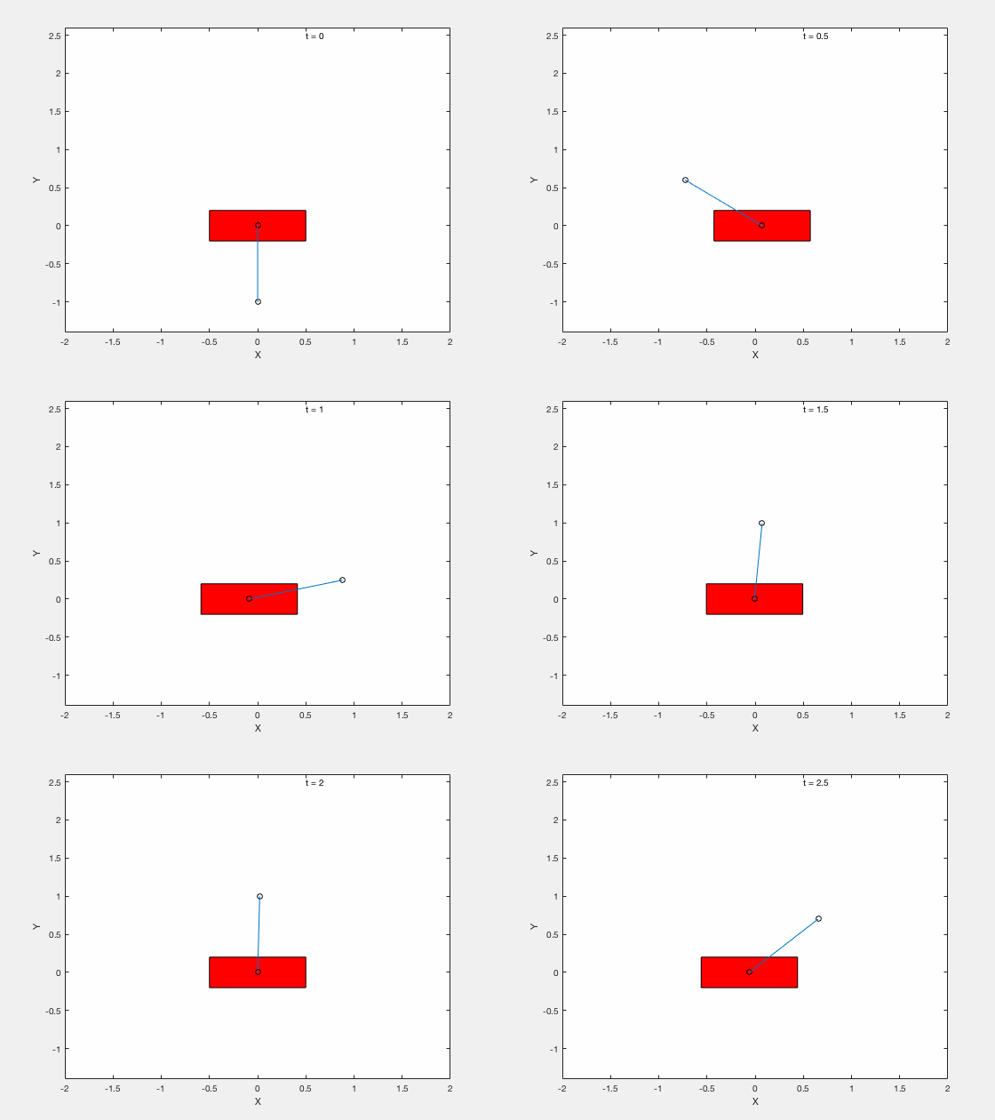
We next apply techniques developed for control of the classical cart-pole problem. All the code can be downloaded from google drive

Below is example of trajectory obtained by using the desired trajectory alone,

Below is example of trajectory obtained by using the desired trajectory with a stabilizing high-gain control applied about this trajectory.