Lyapunov methods

(NEEDS REVISION)

Vivek Yadav, PhD

We previously saw how nonlinear systems can be controlled using linearization about a desired trajectory. We will now derive mathematical conditions under which this linearizing control results in error going to zero.

Linearization and local stability.

As we saw before, linearization can be used to design controllers for local region around some operating point. However, the properties of linearized system need not apply to the nonlinear system. Consider the following 2 nonlinear systems,

$Sys~1: ~ \dot{X} = -X + X^2$ $Sys~2: ~ \dot{X} = -X - X^3$

The linearization of both the systems is

$\dot{X} = -X$

which is stable in local neighborhood of the equilibirum point $ 0 $. However, the true nonlinear system 1 is stable for all $ X<0$ and the second system is stable for all $X$. Therefore, linearizing a nonlinear system tells about local stability of the equilibirum point, but one must be careful in extending these properties to entire state space. As an example consider the following 2 nonlinear systems,

$Sys~1: ~ \dot{X} = -X + X^2$ $Sys~2: ~ \dot{X} = -X + 100 X^2$

Both the systems have the same linearization representation, however, the region in which $\dot{X} < 0$ is different for the two systems. Therefore, the region of stability around $ X=0 $ is different for the two systems. As a final example, consider the two systems,

$Sys~1: ~ \dot{X} = X + X^2$ $Sys~2: ~ \dot{X} = X - X^3$

Linearization of both the systems is $ \dot{X} = X $ which is unstable, however for the second system, \(

\dot{X}

for \(

> 1 \), therefore the states of second system will not diverge to infinity, inspite of them diverging away from 0. In this case 0 is the unstable point, however the states of the full nonlinear system may be bounded.

Therefore, Lyapunov’s linearization method should be interpreted very carefully. ** Lyapunov’s linearization method only describes the behavior of the nonlinear system in a local neighborhood of the linearization (typically equilibirum) point. **

For a nonlinear system described by $ \dot{X} = f(X) $, Lyapunov’s criteria for linearized system states that the system is strictly stable if the linearization

$A = \frac{\partial f}{\partial X}$

is stable.

Lyapunov direct method

We saw that Lyapunov’s linearization method can give some idea of stability about a point. However, it is not sufficient to identify the behavior of the system throughout the state space.

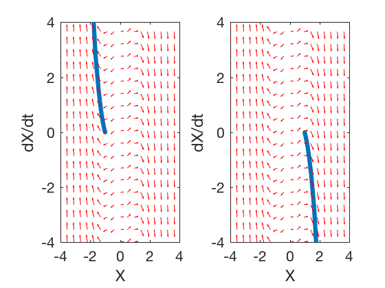
Example 1:

Consider the system,

$\dot{X} = X-X^3$

A Lyapunov function can be written as,

$L(X) = \frac{1}{2}X^TX =\frac{1}{2}X^2$

Taking derivative of the Lyapunov function with respect to time gives,

$\dot{L} = X\dot{X} = X(X-X^3) = X^2(1-X^2)$

The Lyapunov derivative above has the following properties,

$\dot{L} < 0 ~for~|X| > 1$ $\dot{L} > 0 ~for~0<|X|<1$ $\dot{L} = 0 ~for~X = 0,1,-1$

Therefore, the states of the system will go to -1 or 1, if states are in negative or positive half of the plane, and will remain at 0, if states were zero.

clc
close all
clear all

X1_0 = -4:.45:4;
X2_0 = -4:.45:4;

[X1_0,X2_0] = meshgrid(X1_0,X2_0);
mu = 1;
sys_vanderPol = @(t,X)[(X(1)-X(1)^3)];

X0 = [X1_0(1)];
time_span = 0:.1:40;

[time,states] = ode45(sys_vanderPol,time_span,-4);
[time,states1] = ode45(sys_vanderPol,time_span, 4);

dX1  = X1_0;
dX2  = X1_0-X1_0.^3;
dX1 = dX1./sqrt(dX1.^2+dX2.^2);
dX2 = dX2./sqrt(dX1.^2+dX2.^2);

figure;
subplot(1,2,1)
plot(states(:,1),states(:,1)-states(:,1).^3,'linewidth',3)
hold on
quiver(X1_0,X2_0,dX1,dX2,.5,'r')
axis([-4 4 -4 4])
xlabel('X');
ylabel('dX/dt');
subplot(1,2,2)
plot(states1(:,1),states1(:,1)-states1(:,1).^3,'linewidth',3)
hold on
quiver(X1_0,X2_0,dX1,dX2,.5,'r')
axis([-4 4 -4 4])
xlabel('X');
ylabel('dX/dt');

Lyapunov stability (energy interpretation)

Lyapunov function choice crucial in designing control system and studying the behavior of nonlinear systems. It is not always possible to idenfity a good candidate for Lyapunov function. However, in physical systems, energy of a system is a good candidate for Lyapunov function. Below are 2 examples of how energy can be used as a candidate for Lyapunov function.

Example 1: Nonlinear spring mass damper.

Consider the nonlinear spring mass damper system given by,

$m \ddot{X} + b|\dot{X}| \dot{X} + k_1 X + k_2 X^2 = 0$

The total energy of the system can be written as,

$E(X,\dot{X}) = \frac{1}{2} m \dot{X}^2 + \int_0^X (k_1 X + k_2 X^2) dX$

Taking the derivative gives,

$\dot{E} = m \dot{X} \ddot{X} + (k_1 X + k_2 X^2) \dot{X}$

substituting $ m \ddot{X} $ from system dynamics equation gives,

$\dot{E} = \dot{X} (- b |\dot{X}| \dot{X} - (k_1 X + k_2 X^2) ) + (k_1 X + k_2 X^2) \dot{X} = - b |\dot{X}| \dot{X}^2$

Therefore, rate of change of energy is equal to the energy dissipated by the damper, and if $ b > 0 $, the system’s states will go to zero.

Example 2: Robot joint control.

Consider the task of designing a set-point controller for a planar robot whose dynamics are given by,

$M(q) \ddot{q} + C(q,\dot{q}) \dot{q} + G(q) = u$

Consider a Lyapunov function of the form,

$L(q,\dot{q}) = \frac{1}{2} \dot{q}^T M(q) \dot{q} + \frac{1}{2}e^T K_p e + V(q)$

where $ e = q - q_d $ is the error between current pose and desired pose. $ V(q) $ is the potential energy of the system, and is related to $ G $ as,

$G(q) = \frac{ \partial V}{\partial q}$

Taking derivative of the Lyapunov function,

$\dot{L} = \dot{q}^T M(q) \ddot{q}+\frac{1}{2}\dot{q}^T \dot{M}(q) \dot{q} + \dot{q}^T K_p e + \dot{q}^T \frac{ \partial V}{\partial q}$ $\dot{L} = \dot{q}^T (u - C(q,\dot{q}) \dot{q} - G(q) )+\frac{1}{2}\dot{q}^T \dot{M}(q) \dot{q} + \dot{q}^T K_p e + \dot{q}^T G(q)$ $\dot{L} = \dot{q}^T (u + K_p e)+\frac{1}{2}\dot{q}^T ( \dot{M}(q) - 2 C(q,\dot{q})) \dot{q}$

Note, for robotic manipulators, $ \dot{M} - 2C $ is a skew symmatric matrix, therefore,

$\dot{q}^T ( \dot{M}(q) - 2 C(q,\dot{q})) \dot{q} = 0$

The Lyapunov function’s derivative therefore becomes,

$\dot{L} = \dot{q}^T (u + K_p e)$

Choosing $ u = - K_p e - K_d \dot{q} $ gives,

$\dot{L} = - \dot{q}^T K_d \dot{q}$

Therefore $ L $ is decreasing for all values of $ \dot{q} $, and is equal to 0 only if $ \dot{q} = 0. $.

In the example above we assumed a fixed set point, however, the same technique can be extended for tracking a time-varying trajectory.

High gain control around a desired trajectory.

Consider the system given by,

$\dot{X} = f(X) + g(X) u$

Say we have a desired trajectory that satisfies,

$\dot{X}_d = f(X_d) + g(X_d) u_d$

The error dynamics between the actual trajectory and the desired trajectory can be written as,

$\dot{X} - \dot{X}_d = f(X) - f(X_d) + g(X)u - g(X_d) u_d$

Assuming,

$e = X - X_d$ $\delta u = u - u_d$

The linearization of the system above gives,

$\dot{e} = \left( \frac{\partial f}{\partial X} + \frac{\partial g(x) u }{\partial X} \right)_{X_d,u_d} e + g(X_d) \delta u + H.O.T$

where $ H.O.T $ represents higher order terms, assuming control $ \delta u = - K e $, the $ H.O.T $ can be written as $ H.O.T = \Delta e $, where $ \Delta e $ is a nonlinear function that represents linearization error. Therefore, the system above can be written as,

$\dot{e} = A(X_d,u_d) e - B(X_d) K e + \Delta = \left( A(X_d,u_d) - B(X_d) K \right) e + \Delta e$

We now set up a Lyapunov function,

$L = \frac{1}{2} e^T e$

Taking derivative of the Lyapunov function gives,

$\dot{L} = e^T \dot{e} = e^T \left( \left( A(X_d,u_d) - B(X_d) K \right) e + \Delta \right)$

Say in a $ \epsilon $ neighborhood of $X_d $, the linearization error \(

\Delta

< \gamma \), therefore,

$\dot{L} \leq -\lambda_{min} e^Te + e^T\Delta e \leq -\lambda_{min} |e|^2 + |e|^2|\Delta| \leq -\lambda_{min} |e|^2 + |e|^2 \gamma = -\lambda_{min} |e|^2 \left( 1 - \frac{\gamma}{\lambda_{min}} \right)$

Therefore, by choosing $ K $ such that the minimum eigen value of $ A - BK $ satisfies,

$\left( 1 - \frac{\gamma}{\lambda_{min}} \right) \geq 0,$

the resulting control law always drives the error between desired and true trajectory to zero. Note, in practice, the linearization error itself depends on the controller gain $K$, therefore we choose a very high $ K $ to ensure that the deviations from linearized trajectory are small, and $ \lambda_{min} $ is much greater than $ \gamma $.