Pres_SystemDynamics slides

System dynamics and state space representation¶

Vivek Yadav¶

MEC 560, 9/12/2016.¶

Outline¶

System dynamics: Definitions and utility
System dynamics modeling considerations
Types of system dynamics models
State space representations: Nonlinear and linear systems,

System dynamics: Definition¶

Definition¶

Definition: System dynamics is a mathematical approach to understanding the behavior of complex systems over time. This typically involves developing equations to represent how variables describing the system evolve.

System dynamics: Utility¶

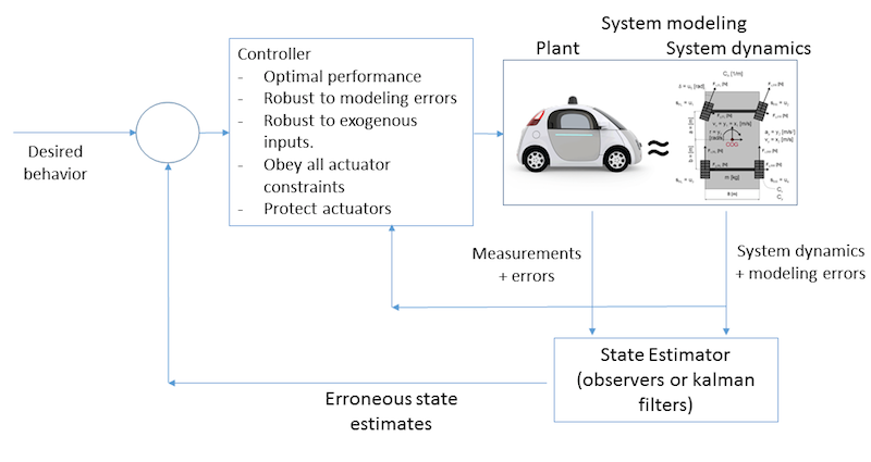
System dynamics allow a control designer to predict how the plant or a system responds to actuator commands and external disturbances.
System dynamics are used to design optimal control signals and observers to estimate variables that define the current state of the system.

System dynamics modeling considerations¶

“All models are wrong, some are useful” ~ George Box.

It is not possible nor is necessary to design a detailed model of the system that we wish to control. The system modeling process often involves several simplifying assumptions. This leads to an important question How much detail is enough for modeling?

Two extremes

Too simple: Does not characterize the actual behavior of the system, can lead to erroneous and potentially adverse control laws.
Too complex: Involves many parameters to specify the model, computationally intractable, and less robust.

System dynamics modeling considerations: Car example¶

Equations of motion of a car

Point mass model $ \ddot{x} = \frac{F}{m} $
Unicycle model $ \dot{v} = \frac{F}{m}, $ and $ \ddot{\theta} = \frac{\tau}{I} $ with the kinematic constraints, $ \dot{x} = v cos(\theta) $ and $ \dot{y} = v sin(\theta) $
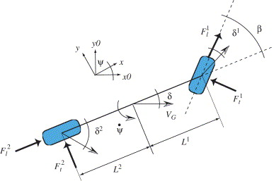
Bicycle model

Side note: Using different system dynamics model for different tasks of the controller.¶

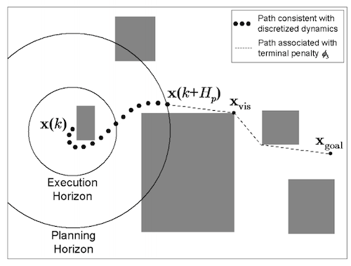
Use different models for different aspects of control (receding horizon control example).

Simple point mass model or ignore dynamics completely to compute obstacle free path
Compute 'feasible' path by approximating dynamics with simpler model with contraints on magnitude of control
Tracking control using a more detailed model

Types of system dynamics models: Continuous, discrete and hybrid¶

Continuous models: Continuous system dynamic models are models that are continuous in time. Such models are described using differential equations.
Discrete models: Discrete system dynamic models are models that are discrete in time, where values describing the system are defined at fixed intervals of time.
Hybrid models: In some cases, it is not possible to describe the system using either continuous or discrete models, and both are required to capture what the system is doing. Example, walking, running, bouncing ball, etc.

State space representations: Definition¶

State-space representation is a mathematical model of a physical system as a set of input, output and state variables related by first-order differential (or difference) equations. ‘State space’ refers to the multi-dimensional space spanned by the state variables. The state of the system can be represented as a vector within this space.

State space representations: More definitions¶

State variables: The state variables are a set of system variables that can completely describe the system at any given time. If the state variables are chosen such that they represent a smallest possible number of variables requires to completely describe the system, then the number of state variables is equal to the order of the system.
Input variables: Input variables refer to the control signals or user applied inputs to the system.
Output variables: Output variables refer to the measurement signals that are used to monitor the plant.
First-order differential (or difference) equations: First order differential equations relate variables to their first order derivatives, and first order difference equations relate values at current time-step to the next.

If the states satisfy an additional contraint on that given the current state of the system, the future states of the system are completely determined by the current state and applied control input. The system dynamics described in this way is memoryless, i.e. the future states do not depend on the past state history or how the current state was achieved. Such processes are also refered as Markov processes (for continuous time) or Markov chains (for discrete time). In cases where the system dynamics is of second order, we split the second order equations into two first order equations.

State space representations: Nonlinear systems¶

continuous nonlinear system¶

$$ \dot{x} = f(x,u), $$

$$ y = h(x,u), $$

If the system dynamics can be expressed as

$$ \dot{x} = f(x) + g(x) u, $$

the system is called control-affine.

Discrete nonlinear system¶

$$ x[k+1] = f(x[k],u[k]), $$

and

$$ y[k] = h(x[k],u[k]). $$

A control affine discrete system can be represented as, $$ x[k+1] = f(x[k]) + g(x[k]) u[k] $$

State space representations: Linear systems¶

Continuous time linear system dynamics model:¶

Continuous time linear system dynamics are modeled as,

$$ \dot{x} = A(t) x(t) + B(t) u(t), $$

where $ A(t) $ is called the system matrix and $ B(t) $ is called the input matrix. Measurements in this case are given by

$$ y(t) = C(t) x(t) + D(t) u(t) ,$$

and $ C(t) $ is the output matrix and $ D(t) $ is the feedforward matrix.

If the matrices are time-invariant, we get Linear Time-Invariant (LTI) systems

$$ \dot{x} = A x(t) + B u(t), $$

$$ y(t) = C x(t) + D u(t) .$$

State space representations: Example¶

$$ \ddot{x} = \frac{F}{m} $$

Define 2 variables, position and velocity.

$$ x_1 = x $$$$ x_2 = \dot{x}_1 = v $$$$ \dot{x}_2 = \frac{F}{m} . $$

System dynamics:

$$ \underbrace{\frac{d}{dt} \left[ \begin{array}{c} x_1 \\ x_2 \end{array} \right]}_{\dot{X}} = \underbrace{\left[ \begin{array}{cc} 0 & 1 \\ 0 & 0 \end{array} \right]}_A \underbrace{\left[ \begin{array}{c} x_1 \\ x_2 \end{array} \right]}_X + \underbrace{\left[ \begin{array}{c} 0 \\ \frac{1}{m} \end{array} \right]}_B \underbrace{F}_u $$

Measurements: positon $ (x) $ and force $ (F) $,

$$ y_1 = x$$$$ y_2 = F$$

Measurements:

$$ y = \underbrace{\left[ \begin{array}{cc} 1 & 0 \\ 0 & 0 \end{array} \right]}_C \underbrace{\left[ \begin{array}{c} x_1 \\ x_2 \end{array} \right]}_X + \underbrace{\left[ \begin{array}{c} 0 \\ 1 \end{array} \right]}_D \underbrace{F}_u $$

State space representations: Linear discrete systems¶

$$ x[k+1] = A x[k] + B u[k], $$

$$ y[k] = C x[k] + D u[k] .$$

State space representations: Hybrid system¶

Hybrid systems are systems that are continous over some interval of time, and discrete over others. One example is a bouncing ball. The equations governing motion of bouncing ball are given by,

$$ \dot{x} = v_x $$

$$ \ddot{y} = -g $$

At impact with ground, the velocity changes as,

$$ \dot{y}^+ = -0.9 \dot{y}^- $$

This is a hybrid system that involves a continuous time formulation for when the ball is in the air, and a discrete time-type of formulation for impact.

Hybrid state-space representation¶

States $ X_1 = x $ , $ X_2 = y $ and $ X_3 = \dot{y} $ with driving inputs $ v_x $ and $ g $.

$$ \dot{X_1 } = v_x $$$$ \dot{X_2 } = X_3 $$$$ \dot{X_3 } = -g $$

At impact, $ X_3^+ = - 0.9 X_3^- $

State space representations: Linearization¶

Why linearize?

Any nonlinear system can be approximated by a linear system under sufficiently stringent assumptions
Linear systems provide computational tools to study the behavior of system
Linearization can be used to identify unstable modes about a stable point and compenstating them using a stabilizing control.

State space representations: Linearization¶

Consider a nonlinear system with an 'equilibrium trajectory' $ x_o, u_o $, such that $ \dot{x}_o = f( x_o, u_o ) $. Small perturbations about this trajectory can be approximated using a simpler linear system.

System dynamics and measurement:

$$ \dot{x} = f(x,u), $$

$$ y = h(x,u), $$

$$ f(x_o+\delta x,u_o+\delta u) \approx f(x_o ,u_o) + \left. \frac{\partial f}{ \partial x} \right|_{(x_o,u_o)} \delta x + \left. \frac{\partial f}{ \partial y} \right|_{(x_o,_o)} \delta u . $$

Derivatives above are derivatives of a vector with respect to a vector.

System dynamics:

$$ \frac{d(x_o + \delta x)}{dt} = \dot{x}_o + \dot{\delta x} \approx f(x_o ,u_o) + \left. \frac{\partial f}{ \partial x} \right|_{(x_o,u_o)} \delta x + \left. \frac{\partial f}{ \partial y} \right|_{(x_o,_o)} \delta u . $$

$$ \dot{\delta x} \approx \left. \frac{\partial f}{ \partial x} \right|_{(x_o,u_o)} \delta x + \left. \frac{\partial f}{ \partial y} \right|_{(x_o,_o)} \delta u . $$

Measurements:

$$ \delta y \approx \left. \frac{\partial h}{ \partial x} \right|_{(x_o,u_o)} \delta x + \left. \frac{\partial h}{ \partial y} \right|_{(x_o,_o)} \delta u . $$

State space representations: Linearization¶

$$ \ddot{\theta} = -\frac{g}{l} sin(\theta) $$

Linearize the system about $ \dot{\theta} = 0 $ and $ \theta = 0 $.

$ x_1 = \theta $ and $ x_2 = \dot{\theta} $

$$ \dot{x}_1 = x_2 $$$$ \dot{x}_2 = -\frac{g}{l} sin(x_1) $$

$$ \frac{d}{dt} \left[ \begin{array}{c} x_1 \\ x_2 \end{array} \right] =\left[ \begin{array}{c} x_2 \\ -\frac{g}{l} sin(x_1) \end{array} \right] = f(x_1, x_2) $$

Taking derivatives,

$$ \frac{\partial f}{\partial x} = \left[ \begin{array}{cc} 0 & 1 \\ -\frac{g}{l} cos(x_1) & 0 \end{array} \right] $$

Derivative at $ x_1 = \theta=0 $ and $ x_2 = \dot{\theta}=0 $ ,

$$ \left. \frac{\partial f}{\partial x} \right|_{0,0}= \left[ \begin{array}{cc} 0 & 1 \\ -\frac{g}{l} cos(0) & 0 \end{array} \right] = \left[ \begin{array}{cc} 0 & 1 \\ -\frac{g}{l} & 0 \end{array} \right] $$

Linearized system is,

$$ \delta \dot{x} = \left. \frac{\partial f}{\partial x} \right|_{0,0} \delta x= \left[ \begin{array}{cc} 0 & 1 \\ -\frac{g}{l} & 0 \end{array} \right] \delta x$$

Applications:¶

Almost all real-world phenomena can be represented using state-space methods. Applications range from predicting regions in brain that are involved in mental processes, developing optimal drug delivary schemes to minimize viral load, parameter estimation for machine learning/artificial intelligence algorithms, and control of self-driven cars and robots. Below are some examples,

Extensions of state space representations¶

State transition function
Markov processes
Baysean networks
Decision networks
Jordan forms
Diagonal form
Canonical form
Minimal representation