Solutions of state space representations

Vivek Yadav

MEC 560, 9/12/2016

Outline

• Solutions of state space representations: Why study linear systems?
• Continuous system
• Discrete system
• Numerical solution
• Examples
• Conclusion

Solutions of state space representations: Linear systems

• Solution method for one linear system applies to all other linear systems. Solution for one nonlinear system, typically does not apply to other nonlinear systems.
• Closed form solution can be obtained for linear systems, which allows us to draw inferences about the behavior of the system
• Closed form solution allows us to test if the underlying process is controllable and observable (to be discussed in the next class).
• Linear systems formulation gives formal techniques to characterize the unstable modes and design controller to cancel those nodes.
• Almost all systems under sufficiently stringent conditions can be approximated as linear system.

Solutions of state space representations: 1st order continuous system

Consider the system given by,

$$ \dot{x} = a x, $$

where \( a \) is a scalar.

Solve for \(x (t) \), given the initial condition \( x_o \)

Solutions of state space representations: Continuous system

System:

$$ \frac{d x(t) }{dt} = A x(t) + B u(t) $$

Special case, \( u = 0 \)

$$ \frac{d x(t) }{dt} = A x(t) $$

Claim: Solution is

$$ x(t) = e^{At} x_o $$

Verify by substitution

$$ \frac{d x(t) }{dt} = \frac{d e^{At} }{dt}x_o $$

Recall

$$ e^{At} = \left ( I + At + \frac{A^2t^2}{2!} + \frac{A^3t^3}{3!} + \dots \right) $$

$$ \frac{de^{At}}{dt} = \left ( A + 2 \frac{A^2 t}{2!} + 3 \frac{A^3 t^2}{3!} + \dots \right) = \left ( A + \frac{A^2 t}{1!} + \frac{A^3 t^2}{2!} + \dots \right) $$

$$ \frac{de^{At}}{dt} = A \left ( I + At + \frac{A^2t^2}{2!} + \frac{A^3t^3}{3!} + \dots \right) = A e^{At}$$

Therefore, $$ \frac{d x(t) }{dt} = \frac{d e^{At} }{dt}x_o =A e^{At} x_o = A x(t)$$

General solution: 1st order continuous system

Consider the system given by,

$$ \dot{x} = a x + bu, $$

where \( a \) is a scalar.

Solve for \(x (t) \), given the initial condition \( x_o \)

General solution: Continuous system

$$ \frac{d x(t) }{dt} = A x(t) + B u(t)$$

with initial condition \( x_o \).

General solution is of the form

$$x(t) = e^{At} c(t)$$

Substituting in \( \dot{x} = Ax + Bu \)

$$ A e^{At} c(t) + e^{At} \frac{d c }{dt} = A e^{At} c(t) + B u(t), $$

Simplifying and rearranging,

$$ \frac{d c }{dt} = e^{-At} B u(t). $$

Integrating with respect to time,

$$ c(t) = \int_{0}^{t} e^{-A \lambda } B u(\lambda) d\lambda + constant. $$

General solution: Continuous system

$$ \frac{d x(t) }{dt} = A x(t) + B u(t)$$

with initial condition \( x_o \).

Solution:

$$x(t) = e^{At} \int_{0}^{t} e^{-A \lambda } B u(\lambda) d\lambda + constant. $$

Using \( x(0) = x_o \),

$$x(t) = x_o + e^{At} \int_{0}^{t} e^{-A \lambda } B u(\lambda) d\lambda. $$

Solution for continuous system

$$x(t) = x_o + e^{At} \int_{0}^{t} e^{-A \lambda } B u(\lambda) d\lambda. $$

• If the eigen values of A have positive real parts, then the system's is unstable and goes to infinity along the directions given by the corresponding eigenvectors.
• If the eigen values of A have negative real parts, the solution goes to 0 asymptotically.
• CAUTION: In MATLAB, DO NOT USE exp(A) to solve for exponential of a matrix, USE expm(A) instead.

• Control \( u \) can be chosen to make the effective eigen values of the system negative. This process is also called pole placement.

Solutions of state space representations: 1st order discrete system

Consider the system given by

$$ x[k+1] = a x[k] $$

Solve for \(x[k]\) given the initial condition \(x_o \).

When u[k] = 0

When $u[k] = 0$, the system dynamics reduces to,

$$ x[k+1] = A x[k] $$

with initial condition \( x[0] = x_o \).

Claim, solution is,

$$ x[k] = A^{k} x_o$$

Verify by substitution,

$$ x[k+1] = A^{k+1} x_o = A (A^{k}x_o) = A x[k]. $$

General case: 1st order discrete system

Consider the system given by,

$$ x[k+1] = a x[k] + bu[k], $$

where \( a \) is a scalar.

Solve for \(x[k] \), given the initial condition \( x_o \)

General case: Discrete system

$$ x[k+1]=Ax[k] + B u[k]$$

with initial condition x[0]=xo.

Claim, solution is, $$ x[k] = A^{k} x[0] + \sum_{i=0}^{k-1}A^{k-i-1} B u[i] $$

Verify by substitution

$$ x[k+1] = A \left( A^{k} x[0] + \sum_{i=0}^{k-1}A^{k-i-1} B u[i] \right) + B u[k] = A^{k+1} x[0] + \sum_{i=0}^{k-1}A^{k-i} B u[i] + B u[k]$$$$ x[k+1] = A^{k+1} x[0] + \sum_{i=0}^{k}A^{k-i} B u[i]$$

$$ x[k+1]=Ax[k] + B u[k]$$

with initial condition x[0]=xo.

$$ x[k] = A^{k} x[0] + \sum_{i=0}^{k-1}A^{k-i-1} B u[i] $$

Properties,

1. The solution for $x[k]$ depends only on the control signals between 0 and current time instant (k).
2. The solutions for $x[k]$ are bounded if $A^{k}$ is bounded is no longer valid, because the solution depends on $B$ and control history $u[k]$ also.

Relation between continuous and discrete representations

$$ \frac{d x(t) }{dt} = A x(t) + B u(t) $$$$ y(t) = C x(t) + D u(t).$$

Discretize the continuous system $$\frac{x[t+\Delta t] - x[t]}{\Delta t} = A x(t) + B u(t) $$

$$x[t+\Delta t] = (I+ A \Delta t) x(t) + B\Delta t u(t) $$

If all the eigen values of $A$ have negative real parts, then the eigen values of $(I+ A \Delta t)$ for a small $\Delta t$ are have real parts less than 1, and $e^{At}$ or $(I+ A \Delta t)^k$ both will converge to $0$ as $t,k \rightarrow \infty $.

Solutions of state space representations: Numerical

It is not always possible to obtain a closed form solution, in such cases numerical methods are employed.

Example: Consider the system \( \dot{x} = a x \) discretized as,

$$ x[k+1] = (1+a \delta t ) x[k] $$

Recall, \( \dot{x} = a x \)'s solution is \( x(t) = x(0)e^{at} \)

clc;close all;clear all
a = -1;x(1) = 1; % x(0)
dt = .2;t(1) = 0;t_f = 2;
N = round(t_f/dt);
for i = 2:N+1
    t(i) = t(i-1) + dt;
    x(i) = (1+a*dt)*x(i-1);
end
figure;
plot(t,x,'ro',t,exp(a*t),'ks')
hold on
plot(t,x,'r',0:.01:t_f,exp(a*(0:.01:t_f)),'k')
ylabel('x');xlabel('t')

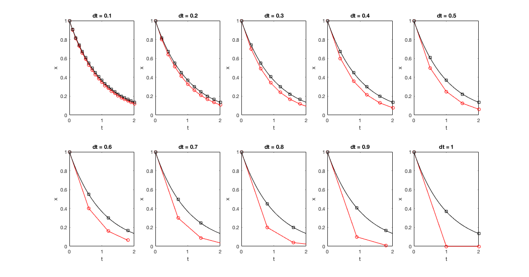
Numerical solutions: Effect of changing dt.

Numerical solutions: Practical guidelines

1. Using smaller 'dt' results in more accurate solution. However, most systems do not have closed form solutions, so we choose a small 'dt'.
2. In practice keep reducing 'dt' by a factor of 2 until no significant change in the solution occurs.
3. Use other numerical techniques to discretize and integrate the system. For example, trapeziod, central difference, Fourth-order Runge-Kutta method to discretize the system.
4. Use ode45 in MATLAB to obtain numerical solutions.
5. You can also solve the equations in linear case directly using expm function on the system dynamics matrix A.

clc;close all;clear all

a = -1;x0 = 1; % x(0)
t_f = 2;
sys_fun = @(t,x)( a * x);
[t,x] = ode45(sys_fun,[0 t_f],x0);

figure;
plot(t,x,'ro',t,exp(a*t),'ks')
hold on;
plot(t,x,(0:0.01:t_f),exp(a*(0:0.01:t_f)),'k')
ylabel('x')
xlabel('t')
title('Solution from ODE45')

State space solution: Numerical for nonlinear systems

For most nonlinear systems, numerical methods are the only way to obtain solution. In such cases, always use higher order integration method such as ode45.

Example: Van der pol oscillator

Van der pol oscillator

$$ \ddot{y} - \mu (1 - y^2) \dot{y} + y = 0 $$

State-space representation:

$$ \dot{y}_1 = y_2 $$$$ \dot{y}_2 = \mu (1 - y_1^2) y_2 - y_1 $$

clc;close all;clear all

mu = 1;
vdp = @(t,y)[y(2); mu*(1-y(1)^2)*y(2)-y(1)];
[t,y] = ode45(vdp,[0 10],[2; 0]);

plot(t,y(:,1),'-o',t,y(:,2),'-o')
title('Van der Pol solution with ODE45');
xlabel('t');
ylabel('y');
legend('y_1','y_2')

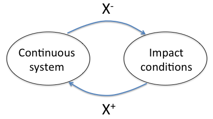
Example: Hybrid system, Bouncing ball

Equations of motion of bouncing ball are given by,

$$ \dot{x} = v_x $$

$$ \ddot{y} = -g $$

At impact with ground, the velocity changes as,

$$ \dot{y}^+ = -0.9 \dot{y}^- $$

This is a hybrid system that involves a continuous time formulation for when the ball is in the air, and a discrete time-type of formulation for impact.

Example: Hybrid system, Bouncing ball

Define state space representation

States \( X_1 = x \) , \( X_2 = y \) and \( X_3 = \dot{y} \) with driving inputs \( v_x \) and \( g \).

$$ \dot{X_1 } = v_x $$$$ \dot{X_2 } = X_3 $$$$ \dot{X_3 } = -g $$

At impact, \( X_3^+ = - 0.9 X_3^- \)

Solution procedure : ODE45 with hybrid conditions,

% System dynamics
function dx = eqn_bouncing_ball(t,x,g,vx)

x1 = x(1);
x2 = x(2);
x3 = x(3);

dx1 = vx;
dx2 = x(3);
dx3 = -g;

dx = [dx1;dx2;dx3];

% Impact condition 
function [value, isterminal, direction] = hit_event(t,x)

% value of variable to keep track of
% isterminal, 1 to stop, 0 otherwise. 
% direction, 
% 0- all zeros of the solution
% 1- only zeros where the event function is increasing
% -1 - only zeros where the event function is decreasing

value = x(2);
isterminal = 1; % 
direction = -1; % decreasing

clc;close all;clear all;

vx = .2;vy = 1;g = 9.81;
options = odeset('Events',@hit_event, 'RelTol',1e-8,'AbsTol',1e-10);
x_0 = [0;0;vy];
t_start = 0;
X_all = [];t_all = [];
for i = 1:10;
    % Integrating continuous system until impact
    [t,X] = ode45(@(t,x)eqn_bouncing_ball(t,x,g,vx), [t_start:0.01:t_start+10],x_0,options);
    X_all = [X_all ; X];
    t_all = [t_all; t];
    % Impact condition
    x_0 = X_all(end,:);
    x_0(3) = -0.9*x_0(3);
    t_start = t(end);
end

ODE45 for bouncing ball

Conclusion

• Solutions of state space representations: Why study linear systems?
• Continuous system
• Discrete system
• Numerical solution
• Examples