Recap
- State space representation
- Controllability
- Pole-placement for different control applications
- Optimal control formulation
- Linear quadratic regulator (LQR) control formulation (first variance principles)
- Dynamic programming for LQR
- Path planning
- LQR using dynamic programming
- Multiple shooting
Outline
- Optimization under constraints
- Direct collocation/Direct transcription
- GPOPs II
Revisiting multiple shooting
- Approximate control using piecewise linear functions
- States approximated at boundary points,
- Dynamic imposed as equality constraints
Characteristics of multiple shooting
- Accurate, because we integrate the dynamics forward
- Dynamics satisfied at all points
- Slow because integrating dynamics is a slow process
- Alternate approach, derivative based direct collocation
Direct collocation: Overview
- Approximate control and state trajectories as piecewise polynomial at some knot points
- Express optimal control problem as a nonlinear program
- Impose equality constraint on the derivative of the polynomial and system dynamics
- Solve the nonlinear program
Direct collocation: Applications
- Fast direct multiple shooting algorithms for optimal robot control
- 3D dynamic walking with underactuated humanoid robots: A direct collocation framework for optimizing hybrid zero dynamics
- On-line path planning for an autonomous vehicle in an obstacle filled environment
- Survey of direct transcription for low-thrust space trajectory optimization with applications
- Optimal control of flexible space robots using direct collocation method and nonlinear programming
- Optimal path planning of UAVs using direct collocation with nonlinear programming
- A survey of numerical methods for optimal control
Direct collocation: Components
Direct collocation involves 3 main components that define the type of direct collocation method,
- Choice of piece-wise polynomial to represent state and control: For states, piecewise cubic polynomials are a good choice. However, depending on the specific problem domain, some methods may be preferred over another. For example, in trajectory optimization of walking robots, Bezier polynomials, in other application Legendre polynomials may be preferable.
- Method of integrating cost function: Cost function is typically chosen as an integral term that depends on the entire trajectory. The integration process can be converted to summation using a fewer intermediate values. The method of numerical integration is also called quadrature.
- Method of state-propogation between time points: In addition to integrating the total cost, we need to integrate from the start of interval to some other point.
Direct collocation (Hermite-Simpson collocation method)
Nonlinear program set up
- Approximate control as piecewise linear functions
- Approximate state trajectory with piecewise continuous cubic polynomials defined by state and derivatives computed from system dynamics at the transition or knot points.
- Calculate derivative from polynomial approximation and from system dynamics at the midpoint and impose equality constraint to drive the error between them to 0.
- Use numerical integration (quadrature) method to approximate the objective function as function of values at knot points
- Express additional equality and inequality constraints as constraints at the collocation points.
Solve the nonlinear program to minimize the objective function subject to dynamics conctraints at collocation points, and any other problem constraints.
Direct collocation: Nonlinear program set up
Minimize,
$$ J(u) = \Phi(X_f) + \int_{t=0}^{t_f} L(t,X,u) dt . $$Subject to,
$$ \dot{X} =f(x,u), $$with initial condition \( X(0) = X_0 \), under constraints,
$$ u_{min} \leq u \leq u_{max}, $$ $$ X_{min} \leq X \leq X_{max}, $$ $$ C_{eq}(X,u) = 0 , $$ $$ C(X,u) \leq 0 , $$We solve this problem using Hermite-Simpson collocation method.
Hermite-Simpson collocation method: Step 1, Discretize
Discretize time \( t_f \) into \( N \) intervals as,
$$ t_0 = 0 \leq t_1 \leq t_2 \leq \dots \leq t_{k} \leq t_{k+1} \dots \leq t_{N}=t_f $$The states between \( tk \) and \( t{k+1} \) can be written as,
$$ X(t) = a_{k,0} + a_{k,1} t + a_{k,2} t^2 + a_{k,3} t^3 , $$which gives
$$ \dot{X}(t) = a_{k,1} + 2 a_{k,2} t + 3 a_{k,3} t^2 , $$where \( a{k,0} \), \( a{k,1} \), \( a{k,2} \) and \( a{k,3} \) are coefficients of the polynomial approximation in \( k^{th} \) interval.
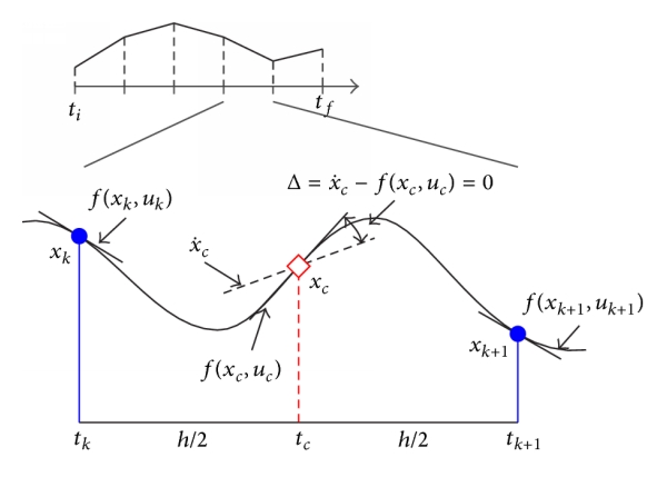
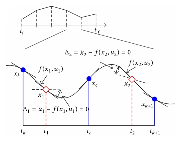
Hermite-Simpson collocation method: Step 2, Compute state derivatives at the collocation point
Collocation point
$$ t_{k,c} = \frac{t_k+t_{k+1}}{2} $$Shift time interval from 0 to h,
$$ X(0) = X_k $$ $$ X(h) = X_{k+1} $$$$ \dot{X}(0) = \dot{X}_{k} = f(X_k,u_k)$$$$ \dot{X}(h) = \dot{X}_{k+1} = f(X_{k+1},u_{k+1}) $$Computing states and derivatives from polynomial approximation,
$$ \left[ \begin{array}{c} X(0) \\ \dot{X}(0) \\ X(h) \\ \dot{X}(h) \end{array} \right] = \left[ \begin{array}{cccc} 1 & 0 & 0 & 0 \\ 0 & 1 & 0 & 0 \\ 1 & h & h^2 & h^3 \\ 0 & 1 & 2 h & 3 h^2 \end{array} \right] \left[ \begin{array}{c} a_{k,0} \\ a_{k,1} \\ a_{k,2} \\ a_{k,3} \end{array} \right] $$Take inverse to compute coefficients.
$$ \left[ \begin{array}{c} a_{k,0} \\ a_{k,1} \\ a_{k,2} \\ a_{k,3} \end{array} \right] = \left[ \begin{array}{cccc} 1 & 0 & 0 & 0 \\ 0 & 1 & 0 & 0 \\ -\frac{3}{h^2} & -\frac{2}{h} & \frac{3}{h^2} & -\frac{1}{h} \\ \frac{2}{h^3} & \frac{1}{h^2} & -\frac{2}{h^3} & \frac{1}{h^2} \end{array} \right] \left[ \begin{array}{c} X(0) \\ \dot{X}(0) \\ X(h) \\ \dot{X}(h) \end{array} \right] $$Using polynomial approximation, compute derivative at collocation point
$$ X_c = X \left( \frac{h}{2} \right) = \frac{1}{2} \left( X_k + X_{k+1} \right) + \frac{h}{8} \left[ f(X_k,u_k) - f(X_{k+1},u_{k+1}) \right] $$ $$ \dot{X}_c = \dot{X} \left( \frac{h}{2} \right) = - \frac{3}{2 h} \left( X_k - X_{k+1} \right) - \frac{1}{4} \left[ f(X_k,u_k) + f(X_{k+1},u_{k+1}) \right] $$Control at midpoint is,
$$ u_c = \frac{u_k+u_{k+1}}{2} $$Defect,
$$ \Delta_k = \dot{X}_c - f(X_c, u_c) $$ $$ \Delta_k = - \frac{3}{2 h} \left[ \left( X_k - X_{k+1} \right) + \frac{h}{6} \left[ f(X_k,u_k) + 4 f(X_c, u_c)+ f(X_{k+1},u_{k+1}) \right] \right] $$We redefine the constraint as,
$$ \Delta_k = \left[ \left( X_k - X_{k+1} \right) + \frac{h}{6} \left[ f(X_k,u_k) + 4 f(X_c, u_c)+ f(X_{k+1},u_{k+1}) \right] \right] $$Term in bracket is integral from Hermite-Simpson approximation when the dynamic constraints are satisfied. This technique results in implicit Hermite-Simpson integration.
3. Express cost-function in terms of optimization parameters.
$$ J(u) = \Phi(X_f) + \int_{t=0}^{t_f} L(t,X,u) dt . $$Using trapezoid integration:
$$ J_{nlp} = \Phi(X_{N}) + \frac{1}{2}\sum_{k=1}^{N-1} \left( L(t_{k+1},X_{k+1},u_{k+1}) + L(t_k,X_k,u_k) \right)(t_{k+1}-t_k) . $$For linear quadratic regulator, with time points discretized evenly at intervals of \( h \):
$$ J_{nlp} = \Phi(X_{N}) + \frac{1}{2}\sum_{k=1}^{N-1} \left( X_{k+1}^T Q X_{k+1} + u_{k+1}^T R u_{k+1} +X_{k}^T Q X_{k} + u_{k}^T R u_{K+1} \right) h. $$4. Define additional constraints
The constraints on states and controls can be expressed as
$$ u_{min} \leq u_k \leq u_{max}, $$ $$ X_{min} \leq X_k \leq X_{max}, $$ $$ C{eq}(X_k,u_k) = 0 , $$ $$ C(X_k,u_k)\leq 0 , $$Problem formulation: Nonlinear programming
$$ \underbrace{minimize}_{X_k,u_k} \left( \Phi(X_{N}) + \frac{1}{2}\sum_{k=1}^{N-1} \left( X_{k+1}^T Q X_{k+1} + u_{k+1}^T R u_{k+1} +X_{k}^T Q X_{k} + u_{k}^T R u_{K+1} \right) h. \right) $$Subject to,
$$ \Delta_k = \left[ \left( X_k - X_{k+1} \right) + \frac{h}{6} \left[ f(X_k,u_k) + 4 f(X_c, u_c)+ f(X_{k+1},u_{k+1}) \right] \right] = 0 $$ $$ u_{min} \leq u_k \leq u_{max}, $$ $$ X_{min} \leq X_k \leq X_{max}, $$ $$ C{eq}(X_k,u_k) = 0 , $$ $$ C(X_k,u_k)\leq 0. $$- No integrals are computed
- Very fast convergence
%% Constraint function
function [C,Ceq]=cons_fn(X_opt)

N = (length(X_opt)-1)/3;
N_st = 2;
t_f = X_opt(1);
x = X_opt(N+2:end);
u = X_opt(2:N+1);
x = reshape(x,N,N_st);
t = linspace(0,1,N)'*t_f;
dt = t(2) - t(1);

tc = linspace (t(1)+dt/2,t(end)-dt/2,N-1);
xdot = innerFunc(t,x,u);
xll = x(1:end-1,:);
xrr = x(2:end,:);
xdotll = xdot(1:end-1,:);
xdotrr = xdot(2:end,:);
ull = u(1:end-1,:);
urr = u(2:end,:);

xc = .5*(xll+xrr)+ dt/8*(xdotll-xdotrr);
uc = (ull+urr)/2;
xdotc = innerFunc(tc,xc,uc);
Ceq = (xll-xrr)+dt/6*(xdotll +4*xdotc +xdotrr );
Ceq =  Ceq(:);

Ceq = [Ceq ;
    x(1,1)-10 ;
    x(end,1);
    x(1,2)
    x(end,2);
    ];
C = [];
%% Cost function

function [cost,grad]= objfun(X_opt)
N = (length(X_opt)-1)/3;
t_f = X_opt(1);
cost = t_f;
grad = zeros(size(X_opt));
grad(1) = 1;
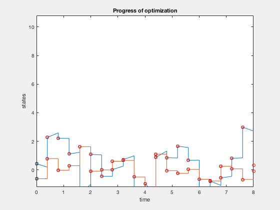
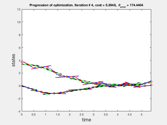
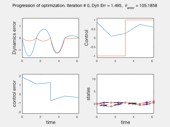
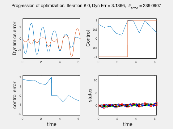
MATLAB DEMO
Solution of direct collocation
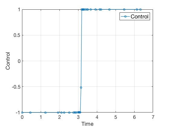
Accuracy of direct collocation method: 5 points
Accuracy of direct collocation method: 21 points
- Accuracy increases as mesh points increase, increasing mesh points to get better solutions is called the p-method
- Direct collocation solution is not accurate, so is used in conjunction with PID control.
Improvements to direct collocation solution
- Higher order collocation methods (p-method)
- Increase number of points (h-method)
- Hybrid methods (Direct and indirect methods): Use necessary conditions and direct collaction together.
- Adaptive grid/mesh: Use non-uniform grid, more points in discontinuous areas
- h, p and hp-methods:
Higher order collocation: Fifth order polynomials
Adaptive mesh
GPOPs II
GPOPs II (pronounced GPOPs 2) is a general purpose optimal control software. GPOPs II stands for, General Purpose OPtimal Control Software version 2. GPOPs' development began in 2007, and the development of GPOPS-II continues today, with improvements that include the open-source algorithmic differentiation package ADiGator and continued development of \(hp\)-adaptive mesh refinement methods for optimal control. Detailed article on GPOPS II and its capibilites can be found here
1. Define bounds on all the variables
%-------------------------------------------------------------------------%
%----------------- Provide All Bounds for Problem ------------------------%
%-------------------------------------------------------------------------%
t0min = 0;  t0max = 0;
tfmin = 0;  tfmax = 200;
x10   = +10; x1f   = 0;
x20   = +0; x2f   = 0;
x1min = -20; x1max =  20;
x2min = -20; x2max =  20;
umin = -1;   umax = +1;

%-------------------------------------------------------------------------%
%----------------------- Setup for Problem Bounds ------------------------%
%-------------------------------------------------------------------------%
bounds.phase.initialtime.lower = t0min;
bounds.phase.initialtime.upper = t0max;
bounds.phase.finaltime.lower = tfmin;
bounds.phase.finaltime.upper = tfmax;
bounds.phase.initialstate.lower = [x10, x20];
bounds.phase.initialstate.upper = [x10, x20];
bounds.phase.state.lower = [x1min, x2min];
bounds.phase.state.upper = [x1max, x2max];
bounds.phase.finalstate.lower = [x1f, x1f];
bounds.phase.finalstate.upper = [x1f, x1f];
bounds.phase.control.lower = [umin];
bounds.phase.control.upper = [umax];
2. Provide initial guess to the solver
%-------------------------------------------------------------------------%
%---------------------- Provide Guess of Solution ------------------------%
%-------------------------------------------------------------------------%
tGuess               = [0; 5];
x1Guess              = [x10; x1f];
x2Guess              = [x20; x2f];
uGuess               = [umin; umin];
guess.phase.state    = [x1Guess, x2Guess];
guess.phase.control  = [uGuess];
guess.phase.time     = [tGuess];
3. Define the mesh and mesh refinement method
%-------------------------------------------------------------------------%
%----------Provide Mesh Refinement Method and Initial Mesh ---------------%
%-------------------------------------------------------------------------%
mesh.method          = 'hp-PattersonRao';
mesh.tolerance       = 1e-6;
mesh.maxiterations    = 20;
mesh.colpointsmin    = 4;
mesh.colpointsmax    = 10;
mesh.phase.colpoints = 4;
4. Set up the problem
%-------------------------------------------------------------------------%
%------------- Assemble Information into Problem Structure ---------------%
%-------------------------------------------------------------------------%
setup.mesh                        = mesh;
setup.name                        = 'Double-Integrator-Min-Time';
setup.functions.endpoint          = @doubleIntegratorEndpoint;
setup.functions.continuous        = @doubleIntegratorContinuous;
setup.displaylevel                = 2;
setup.bounds                      = bounds;
setup.guess                       = guess;
setup.nlp.solver                  = 'ipopt';
setup.derivatives.supplier        = 'sparseCD';
setup.derivatives.derivativelevel = 'second';
setup.method                      = 'RPM-Differentiation';
%% Dynamics

function phaseout = doubleIntegratorContinuous(input)

t  = input.phase.time;
x1 = input.phase.state(:,1);
x2 = input.phase.state(:,2);
u  = input.phase.control(:,1);

x1dot = x2;
x2dot = u;

phaseout.dynamics = [x1dot, x2dot];
%% Objective

function output = doubleIntegratorEndpoint(input)

output.objective = input.phase.finaltime;
4. Solve the problem using GPOPS II
%-------------------------------------------------------------------------% %----------------------- Solve Problem Using GPOPS2 ----------------------% %-------------------------------------------------------------------------%
output = gpops2(setup);
States for optimal control computed using GPOPS II.
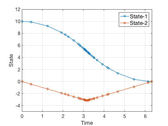
States for optimal control computed using GPOPS II.
Practial tips for optimization
- Cost function: Define cost functions that have smooth derivatives. If the cost function is not smooth, it can be made smooth by modifying the cost function. For example, \( | x | \) can be written as \( \sqrt{X^2 + \epsilon } \) or cost function can be expresses as \( x \) with the constraint that \( x \geq 0 \).
- Initial guess: A good initial guess puts the solver in region of global minima and avoids potentially getting stuck in local minimas. Tips on choosing a good initial guess,
- Initialize states as linear functions between start and end
- Solve the problem for a simpler kinematic model by completely ignoring the dynamics of the plant.
- Solve a simpler problem with simpler cost function first, and then use it as initial guess for the main problem. For example, power is a complex cost function \( |u \dot{x}| \), therefore instead a quadratic cost function can be defined first \( u^2 \), and the solution from this simpler problem can be used as initial guess in the next stage.
- Solve optimization with a small grid size, and use this as input for finer or more advanced mesh types.
- Solve optimization with fewer constraints first, and then solve the full problem with all the constraints included.
- Use experimental data or domain knowledge to specify the initial guess. For example, in human reaching tasks, a minimum jerk trajectory can be a good initial guess for the optimizer.
- Bound constraints: Typically as more bound contraints are included, the solver's search space narrows, and an approximate solution can be found.
- Path contraints: Path constraints can significantly restrict the search space, and lead to infeasible solutions. You may compute a sub-optimal trajectory with fewer path constraints, and then add path constraints with this trajectory as initial guess.
- Derivatives: Always provide analytical derivatives of states and constraints. You may use ADiGator. ADiGator uses forward mode automatic differentiation to generate a new file which contains the calculations required to compute the numeric derivatives of the original user function.