Extended Kalman Filter¶

MEC 560: Advanced Control Systems¶

Vivek Yadav, PhD¶

Overview¶

Observability of nonlinear systems
EKF: Extended Kalman Filter for nonlinear system
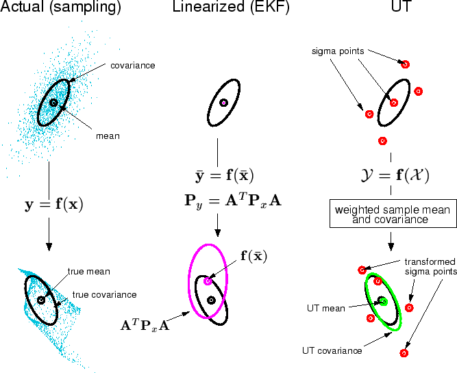
EKF vs UKF

Observability matrix¶

Observability for nonlinear system $ \dot{X} = f(X) + g(X)u $ with measurement $ y = h(x) $ is given by

is given by,

$$ O(f,h) = [ L^0_fh^T~ L^1_fh^T~ L^2_fh^T~ \dots ~ L^{n-1}_fh^T] $$

If the observability matrix above has a full rank, then the states of the system can be estimated. Note, observability matrix may lose rank in some state-space and could potentially become unobservable.

Extended Kalman Filter (EKF)¶

Consider the nonlinear system given by,

$$ X_{k} = f(X_{k-1}) + w_{k-1} $$

with measurement

$$ Z_{k} = h(X_{k}) + v_{k} $$

where $ w_k$ and $ v_k $ represent process and measurement noise with means 0 and covarances given by $Q_k$ and $R_k$. We further assume that state covariance is given by a matrix $ P $. Detailed derivation of extended kalman filter can be found here. The EKF is implemeted in the following steps.

Model and observation¶

Given the model

$$ X_{k} = f(X_{k-1}) + Fw_{k-1} $$

with measurement

$$ Z_{k} = h(X_{k}) + v_{k} $$

Initialization¶

$$ \hat{X}_0 = \mu_0$$$$ P_0 = P_0$$

Forecasting step¶

$$ \hat{X}_{k}^- = f(\hat{X}_{k-1}^+) $$$$ P_{k}^- = \frac{\partial f}{\partial X} P_{k-1}^+ \frac{\partial f}{\partial X}^T + FQ_{k-1}F' $$

where the partial derivatives are evaluate at $ X_{k-1}^+ $.

Correction step¶

$$ K_k = P_{k}^- \frac{\partial h}{\partial X}^T \left( \frac{\partial h}{\partial X} P_{k}^-\frac{\partial h}{\partial X}^T + R_k \right)^{-1}$$$$ P_k^+ = \left( I - K_k \frac{\partial h}{\partial X} \right)P_{k}^- $$

The partial derivatives are evaluated at $ X_{k}^- $.

$$ X_k^+ = X_k^- + K_k(Z_k - h(X_k^-)) $$

Unicycle example:¶

Consider the dynamics of a unicycle car moving along a straight line at angle of 45-degrees.

$$ \dot{x} = V cos(\theta) $$

$$ \dot{y} = V sin(\theta) $$

$$ \dot{\theta} = \omega $$

Discretizing,¶

$$ x_{k+1} = x_k + \delta t(V_k+w_v) cos(\theta) $$

$$ y_{k+1} = y_k +\delta t(V_k+w_v) sin(\theta) $$

$$ \theta_{k+1} = \theta_k + \delta t(\omega_k+w_\omega) $$

Separating noise and state terms gives,¶

$$ \left[ \begin{array}{c} x_{k+1} \\ y_{k+1} \\ \theta_{k+1} \end{array} \right] = \left[ \begin{array}{c} x_k + \delta t V_k cos(\theta) \\ y_k +\delta tV_k sin(\theta) \\ \theta_k + \delta t \omega_k \end{array} \right] + \left[\begin{array}{cc} \delta t cos(\theta) & 0 \\ \delta t sin(\theta) & 0 \\ 0 & \delta t \end{array} \right] \left[\begin{array}{c} w_v \\ w_\omega \end{array} \right] $$

In [3]:

clc
close all
clear all


dt = 0.001;
v = .5;
head_ang = pi/4;


C = [1 0 0;
    0 1 0];
R = diag([.001 .001]);

Q = diag([.1 .01]);
P_pl = eye(3);

X_hat_0 = [0;0;0];
X_0 = [.1;.1;head_ang];
X_hat_0 = X_0/2;


X(:,1)= X_0;
Y(:,1) = C*X(:,1);
t(1) = 0;
X_hat(:,1)= X_hat_0;

In [4]:

for i = 1:4000
    u = [.5;0];
        
    t(i+1) = t(i)+dt;
    % True process
    X(:,i+1)= X(:,i) + dt*[u(1)*cos(X(3,i));
        u(1)*sin(X(3,i));
        u(2);];
    Y(:,i+1) = C*X(:,i+1) + sqrt(R)*randn(size(C,1),1);  %*randn(2,1);
    % Observer model
        
    dFdx = [0 0 -v*sin(X_hat(3,i)); 0 0 v*cos(X_hat(3,i)); 0 0 0 ];
    dFdx_d = eye(3) + dt*dFdx;
    
    F = [dt*cos(X_hat(3,i)) 0;
    dt*sin(X_hat(3,i)) 0;
    0 dt];
    
    P_mi = dFdx_d*P_pl*dFdx_d' + F*Q*F';
       
    X_hat(:,i+1) = X_hat(:,i) + dt*[u(1)*cos(X_hat(3,i));
            u(1)*sin(X_hat(3,i));
          u(2);];
    Y_hat(:,i+1) = C*X_hat(:,i+1);
    % Update based on measurement
    e_Y  = Y(:,i+1) - Y_hat(:,i+1);
    S = C*P_mi*C'+R;
    K = P_mi*C'*inv(S);
    P_pl = (eye(3) - K*C)*P_mi;
    X_hat(:,i+1)=X_hat(:,i+1) + K*e_Y;
end
X_hat(3,1) = X_hat(3,end);
P_pl = P_mi;

In [5]:

figure;
subplot(2,1,1)
plot(t,X(1,:),t,X_hat(1,:),'--')
legend('true','estimate')
%axis([0 2.5 0 40])
xlabel('time')
ylabel('X')
axis([0 4 0 2])
subplot(2,1,2)
plot(t,X(2,:),t,X_hat(2,:),'--')
legend('true','estimate')
xlabel('time')
ylabel('Y')
axis([0 4 0 2])

In [6]:

figure;
plot(t,X(3,:),t,X_hat(3,:),'--')
axis([0 4 0 1])
xlabel('time')
ylabel('Theta')
%axis([0 2.5 0 2])

Conclusion: Extended Kalman filter.¶

Works well for most nonlinear systems
Calculating apriori covariance requires linearization approximation, which may not be true.
For highly nonlinear systems, can result in erroneous estiamtes

Unscented transform¶

Unscented transforms are used to obtain a better estimate of covariance matrix
Choose some sigma points, propagate state and compute new covariance directly

In [ ]: