Linear control principles for control of nonlinear systems

MEC 560: Advanced control systems

Vivek Yadav, PhD

Overview

• Nonlinear systems have very complex dynamics
• Nonlinear systems can be approximated as linear system under special cases
• In such cases, control based on linear scheme can provide stable results.

Control synthesis: General case

Consider the system given by,

$$ \dot{X} = f(X,u) $$

Compute desired trajectory (GPOPS II, or other SW).

$$ \dot{X_d} = f(X_d, u_d) $$

where \(d \) denotes desired trajectory. Taking error between the true and desired system dyanmic equations gives,

$$ \dot{X} - \dot{X_d} = f(X,u) - f(X_d,u_d) $$

Defining \( e = X - X_d \) and \( \delta u = u - u_d \) , gives

$$ \dot{e} = f(X_d+e,u_d+\delta u) - f(X_d,u_d) $$

Taking Taylor series expansion about \(X_d\) gives,

$$ \dot{e} = f(X_d,u_d) + \left. \frac{\partial f}{ \partial X} \right|_{X_d,u_d} e + \left. \frac{\partial f}{ \partial u} \right|_{X_d,u_d} \delta u - f(X_d,u_d) + H.O.T $$

Where HOT stands for higher order terms. Ignoring the higher order terms gives,

$$ \dot{e} = \left. \frac{\partial f}{ \partial X} \right|_{X_d,u_d} e + \left. \frac{\partial f}{ \partial u} \right|_{X_d,u_d} \delta u$$

$$ \dot{e} = A_d e + B_d \delta u$$

where,

$$ A_d = \left. \frac{\partial f}{ \partial X} \right|_{X_d,u_d} $$$$ B_d = \left. \frac{\partial f}{ \partial u} \right|_{X_d,u_d} $$

Final control law,

$$ u = u_d + \delta u $$

Control synthesis for robotic applications

$$ M (q) \ddot{q} + C(q,\dot{q}) \dot{q} + G(q) = \tau $$

• \( M(q) \) for robots is always invertible.

$$ \ddot{q} = M(q)^{-1}ff(q,\dot{q},\tau). $$

The expression above can be linearized about a desired trajectory as,

$$ \ddot{\delta q} = \ddot{q} - \ddot{q}_d \approx \left. \frac{\partial M(q)^{-1} ff}{ \partial q} \right|_{(q_d,\dot{q_d},\tau_d)} \delta q + M(q_d)^{-1} \left. \frac{\partial ff}{ \partial \dot{q}} \right|_{(q_d,\dot{q_d},\tau_d)} \delta \dot{q}+ M(q_d)^{-1} \left. \frac{\partial ff}{ \partial \tau} \right|_{(q_d,\dot{q_d},\tau_d)} \delta \tau$$

$$ \ddot{\delta q} = \left( \left. \frac{\partial M(q)^{-1} }{ \partial q} \right|_{(q_d,\dot{q_d},\tau_d)} \circ ff \right) \delta q + M(q_d)^{-1}\left. \frac{\partial ff}{ \partial q} \right|_{(q_d,\dot{q_d},\tau_d)} \delta q + M(q_d)^{-1} \left. \frac{\partial ff}{ \partial \dot{q}} \right|_{(q_d,\dot{q_d},\tau_d)} \delta \dot{q}+ M(q_d)^{-1} \left. \frac{\partial ff}{ \partial \tau} \right|_{(q_d,\dot{q_d},\tau_d)} \delta \tau$$

where,

$$ \left( \left. \frac{\partial M(q)^{-1} }{ \partial q} \right|_{(q_d,\dot{q_d},\tau_d)} \circ ff \right) $$

is a tensor product between derivative of inverse of \( M(q) \) and \( ff \). Illustration here. The derivative of the inverse of mass matrix can be computed as,

$$ \frac{\partial M(q)^{-1} }{ \partial q} = - M(q)^{-1} \frac{\partial M(q)}{\partial q} M(q)^{-1} $$

and

$$ ff(q,\dot{q},\tau) = (\tau - C(q,\dot{q}) \dot{q} - G(q)), $$

$$ \dot{\delta q}_1 = \delta q_2 $$$$ \dot{\delta q}_2 \approx \left. \frac{\partial M(q)^{-1} ff}{ \partial q} \right|_{(q_d,\dot{q_d},\tau_d)} \delta q_1 + M(q_d)^{-1} \left. \frac{\partial ff}{ \partial \dot{q}} \right|_{(q_d,\dot{q_d},\tau_d)} \delta q_2+ M(q_d)^{-1} \left. \frac{\partial ff}{ \partial \tau} \right|_{(q_d,\dot{q_d},\tau_d)} \delta \tau$$$$ \frac{d}{dt} \left[ \begin{array}{c} \delta q_1 \\ \delta q_2 \end{array} \right] = \left[ \begin{array}{cc} 0 & I\\ \left. \frac{\partial M(q)^{-1} ff}{ \partial q} \right|_{(q_d,\dot{q_d},\tau_d)} & M(q_d)^{-1} \left. \frac{\partial ff}{ \partial \dot{q}} \right|_{(q_d,\dot{q_d},\tau_d)} \end{array} \right] \left[ \begin{array}{c} \delta q_1 \\ \delta q_2 \end{array} \right] + \left[ \begin{array}{c} 0 \\ M(q_d)^{-1} \left. \frac{\partial ff}{ \partial \tau} \right|_{(q_d,\dot{q_d},\tau_d)} \end{array} \right] \tau$$

Considerations

1. Discretized dynamics is not true dynamics, and may be uncontrollable for some combinations of state variables.
2. As desired trajectory is computed under some simplifying assumptions, the desired trajectory neednt follow the true dynamics.
3. Applying a high-gain control about desired trajectory results in good tracking performance of the controller.

Trajectory generation using GPOPS II

1. Define continuous dynamics using derived Equations of motion.
2. Define end constraint (cost)
3. Define bounds on variables.
4. Use GPOPS to compute sub-optimal solution and use it as trajectory to track.

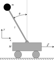
Cart-pole example (MATLAB demo)

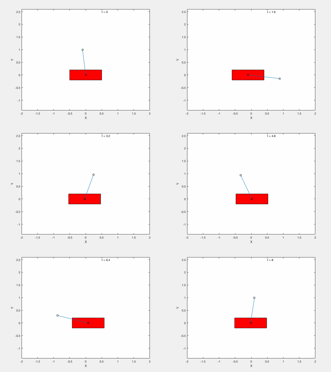
We will test the effectiveness of linearizing control by testing the performance of the controller on following 3 tasks,

1. Stabilize the pendulum about the vertical position.
2. Apply Linear Quadratic Regulator (LQR) to drive the error between the desired and true state to 0.
3. Apply control to move the pendulum from downward position \(x = 0, \theta = pi\) to upright position \( x = 0,\theta = 0\).

Dynamics of cart pole function dq = dynamics_cartpole(t,q)

model_params;

x = q(1);
th = q(2);
dx = q(3);
dth = q(4);

% Generating control based on linearized system:
x_d = 0;
th_d = 0;
dx_d = 0;
dth_d = 0;
u_f_d = 0;

ff_d = ff_cartpole(x_d,th_d,dx_d,dth_d,m_cart,m_mass,l,u_f_d,g);
M_d = M_cartpole(x_d,th_d,dx_d,dth_d,m_cart,m_mass,l,u_f_d,g);
dMdq_d = dMdq_cartpole(x_d,th_d,dx_d,dth_d,m_cart,m_mass,l,u_f_d,g);
dfdq_d = dfdq_cartpole(x_d,th_d,dx_d,dth_d,m_cart,m_mass,l,u_f_d,g);
dfd_dq_d = dfd_dq_cartpole(x_d,th_d,dx_d,dth_d,m_cart,m_mass,l,u_f_d,g);
dfdu_d = dfdu_cartpole(x_d,th_d,dx_d,dth_d,m_cart,m_mass,l,u_f_d,g);

Dynamics of cart pole (contd.)

[A_lin,B_lin] = get_linearized_system(dMdq_d,dfdq_d,dfd_dq_d,dfdu_d,M_d,ff_d);
Q = 10*diag([1 1 1 1]);
R = 0.001;

P = care(A_lin,B_lin,Q,R); % Generate control based on linearized system
K = inv(R)*B_lin'*P;

u_f = -1*K*q;

ff = ff_cartpole(x,th,dx,dth,m_cart,m_mass,l,u_f,g);
M = M_cartpole(x,th,dx,dth,m_cart,m_mass,l,u_f,g);


ddq = M\ff;

dq = [q(3:4);
        ddq];

Simulation

clc
close all
clear all

q = [0;.1;0;0];

t = 0;

dq = dynamics_cartpole(t,q);
time_span = 0:0.1:8;


[time,states] = ode45(@dynamics_cartpole,time_span,q);

Without LQR

With LQR

Generating desrired (sub-optimal) trajectory with GPOPS II

1. Make a continuous function with dynamics and path constraints
2. Make end-point function with cost
3. Set up bounds
4. Solve using GPOPS II

dynamics

function phaseout = cartPoleContinuous(input);


x_all   = input.phase.state(:,1);
th_all  = input.phase.state(:,2);
dx_all  = input.phase.state(:,3);
dth_all = input.phase.state(:,4);
u_all   = input.phase.control(:,1);

dq_all = get_dynamics(x_all,th_all,dx_all,dth_all,u_all);


phaseout.dynamics  = dq_all;
phaseout.integrand = u_all.^2;

Get Dynamics

function dq_all = get_dynamics(x_all,th_all,dx_all,dth_all,u_all)


model_params;

for i = 1:length(th_all);

    th = th_all(i);    
    x = x_all(i);    
    dth = dth_all(i);    
    dx = dx_all(i);
    u_f = u_all(i);
    ff = ff_cartpole(x,th,dx,dth,m_cart,m_mass,l,u_f,g);
    M = M_cartpole(x,th,dx,dth,m_cart,m_mass,l,u_f,g);


    ddq = M\ff;

    dq_all(i,:) = [dx dth ddq'];
end

End point cartpole

function output = cartPoleEndpoint(input)
% input.auxdata.dynamics;


q = input.phase.integral;
tf = input.phase.finaltime;

gamma = input.auxdata.gamma;


output.objective = tf+gamma*q;

Bounds

% setting up bounds
bounds.phase.initialtime.lower  = 0;
bounds.phase.initialtime.upper  = 0;
bounds.phase.finaltime.lower    = 0.001; 
bounds.phase.finaltime.upper    = tf;
bounds.phase.initialstate.lower = [x0 th0 dx0 dth0];
bounds.phase.initialstate.upper = [x0 th0 dx0 dth0];
bounds.phase.state.lower        = xMin;
bounds.phase.state.upper        = xMax;
bounds.phase.finalstate.lower   = [xf thf dxf dthf];
bounds.phase.finalstate.upper   = [xf thf dxf dthf];
bounds.phase.control.lower      = uMin; 
bounds.phase.control.upper      = uMax; 
bounds.phase.integral.lower     = 0;
bounds.phase.integral.upper     = 100000;

Guess

rng(0);

xGuess = [x0;xf]; 
thGuess = [th0;thf]; 
dxGuess = [dx0;dxf]; 
dthGuess = [dth0;dthf];
uGuess = [0;0];
tGuess = [0;tf]; 

guess.phase.time  = tGuess;
guess.phase.state = [xGuess,thGuess,dxGuess,dthGuess];
guess.phase.control        = uGuess;
guess.phase.integral         = 0;

% 

setup.name                        = 'cartpole-Problem';
setup.functions.continuous        = @cartPoleContinuous;
setup.functions.endpoint          = @cartPoleEndpoint;
setup.bounds                      = bounds;
setup.auxdata                     = auxdata;
setup.functions.report            = @report;
setup.guess                       = guess;
setup.nlp.solver                  = 'ipopt';
setup.derivatives.supplier        = 'sparseCD';
setup.derivatives.derivativelevel = 'first';
setup.scales.method               = 'none';
setup.derivatives.dependencies    = 'full';
setup.mesh.method                 = 'hp-PattersonRao';
setup.mesh.tolerance              = 1e-2;
setup.method                      = 'RPM-Integration';

output = gpops2(setup);
output.result.nlptime
solution = output.result.solution;

Tracking using same method as before,

function dq = dynamics_cartpole(t,q)

model_params;

x = q(1);
th = q(2);
dx = q(3);
dth = q(4);

% Generating control based on linearized system:

if (norm(th)<.1 & norm(dth)<1)
    x_d = 0;
    th_d = 0;
    dx_d = 0;
    dth_d = 0;
    u_f_d = 0;
else
    generate_desired_Polynomials;

    x_d = ppval(pp_states.x,t);
    th_d = ppval(pp_states.th,t);
    dx_d = ppval(pp_states.dx,t);
    dth_d = ppval(pp_states.dth,t);
    u_f_d = ppval(pp_controls.u,t);
end

q_d = [x_d;th_d;dx_d;dth_d];

ff_d = ff_cartpole(x_d,th_d,dx_d,dth_d,m_cart,m_mass,l,u_f_d,g);
M_d = M_cartpole(x_d,th_d,dx_d,dth_d,m_cart,m_mass,l,u_f_d,g);
dMdq_d = dMdq_cartpole(x_d,th_d,dx_d,dth_d,m_cart,m_mass,l,u_f_d,g);
dfdq_d = dfdq_cartpole(x_d,th_d,dx_d,dth_d,m_cart,m_mass,l,u_f_d,g);
dfd_dq_d = dfd_dq_cartpole(x_d,th_d,dx_d,dth_d,m_cart,m_mass,l,u_f_d,g);
dfdu_d = dfdu_cartpole(x_d,th_d,dx_d,dth_d,m_cart,m_mass,l,u_f_d,g);


u_f = -[100 100 10 10]*(q -q_d)  + u_f_d;

ff = ff_cartpole(x,th,dx,dth,m_cart,m_mass,l,u_f,g);
M = M_cartpole(x,th,dx,dth,m_cart,m_mass,l,u_f,g);


ddq = M\ff;

dq = [q(3:4);
    ddq];

Without PD control on error term

With PD control on error term