DO NOT use generic names for iterators
for i = 1:10,
     for i = 1:20 % i from above will be rewritten as 20.
         (YOUR CODE)
     end
endclc
close all
clear all
addpath Screws;
addpath fcn_support;
addpath fcn_models;
define_syms;
get_kinematics_cart;
get_EOMs_cart;
linearize_EOM_cart;syms m_cart x dx ddx g 'real'
syms m_mass l th dth ddth 'real'
syms u_th 'real'
vars = {'x','th','dx','dth', ...
'm_cart','m_mass','l','u_th','g'};MATLAB's SYMBOLIC PACKAGE RUNS BEST IN ITS OWN ENVIRONMENT. USING IN MATLAB KERNELS VIA JUPYTER ETC TYPICALLY GIVES ERRORS
%% THIS CODE GIVES ERROR WHEN RAN THROUGH JUPYTER KERNEL.
%% USE MATLAB's NATIVE ENVIRONMENT TO DERIVE EQUATIONS OF MOTION
% Simple example
syms m_cart x dx ddx g 'real'
syms m_mass l th dth ddth 'real'
syms u_th 'real'
Invalid variable name "matrix(0, 1, [])" in ASSIGNIN.
Steps
Identify parameters of your model, masses, link lengths, inertia, center-of-mass etc.
Define kinematics using any method,
If the involved mass is point-mass, then moment of inertia terms are zero, and \(cm\) is at the mass itself.
$$ PE = \sum_{i=1}^N m_i g h_{i,cm} $$\(PE \) is the potential energy of the mass\( ~i \), and \( h_{i,cm} \) is the component along gravity.
where A is a matrix that specifies any additional Pfaffin contraints on the body.
$$ A(q) \dot{q} = 0 $$In cases where there are no constraints, \( A = 0 \).
If you are faimilar with the screw theory based approaches, you can do parts 1 to 3 using the provided scripts in Screws folder
Using the provided script,
[M,C,G] = get_mat(KE_total,PE_total,q_v,dq_v);
gives equations of motion as,
$$ M (q) \ddot{q} + C(q,\dot{q}) \dot{q} + G(q) = \tau $$Define,
$$ ff(q,\dot{q},\tau) = (\tau - C(q,\dot{q}) \dot{q} - G(q)), $$Write \( M(q) \) and \( ff(q) \) to files
write_file(Mr,'M_cartpole.m',vars);
write_file(ffr,'ff_cartpole.m',vars);
Compute accelerations using,
$$ \ddot{q} = M(q)^{-1}ff(q,\dot{q},\tau) $$Taylor series expansion gives,
$$ f(x+\delta x,y+\delta y,z+\delta z) \approx f(x ,y,z) + \left. \frac{\partial f}{ \partial x} \right|_{(x,y,z)} \delta x + \left. \frac{\partial f}{ \partial y} \right|_{(x,y,z)} \delta y + \left. \frac{\partial f}{ \partial z} \right|_{(x,y,z)} \delta z . $$Applying the rule above,
$$ M(q)^{-1}ff(q,\dot{q},\tau) - M(q_d)^{-1}ff(q_d,\dot{q_d},\tau_d) \approx \left. \frac{\partial M(q)^{-1} ff}{ \partial q} \right|_{(q_d,\dot{q_d},\tau_d)} \delta q + M(q_d)^{-1} \left. \frac{\partial ff}{ \partial \dot{q}} \right|_{(q_d,\dot{q_d},\tau_d)} \delta \dot{q}+ M(q_d)^{-1} \left. \frac{\partial ff}{ \partial \tau} \right|_{(q_d,\dot{q_d},\tau_d)} \delta \tau$$Applying chain rule gives,
$$ \left( \left. \frac{\partial M(q)^{-1} }{ \partial q} \right|_{(q_d,\dot{q_d},\tau_d)} \circ ff \right) \delta q + M(q_d)^{-1}\left. \frac{\partial ff}{ \partial q} \right|_{(q_d,\dot{q_d},\tau_d)} \delta q + M(q_d)^{-1} \left. \frac{\partial ff}{ \partial \dot{q}} \right|_{(q_d,\dot{q_d},\tau_d)} \delta \dot{q}+ M(q_d)^{-1} \left. \frac{\partial ff}{ \partial \tau} \right|_{(q_d,\dot{q_d},\tau_d)} \delta \tau$$*** Simple example of \( \circ \) operation in action with the structure of tensor and vectors can be found here
Expression above involves calculation of
$$ \frac{\partial M(q)^{-1} }{ \partial q} . $$Noting,
$$ M(q)^{-1}M(q) = I, $$$$ \frac{\partial M(q)^{-1} }{ \partial q} M(q) + M(q)^{-1} \frac{\partial M(q)}{\partial q} = 0 $$Therefore,
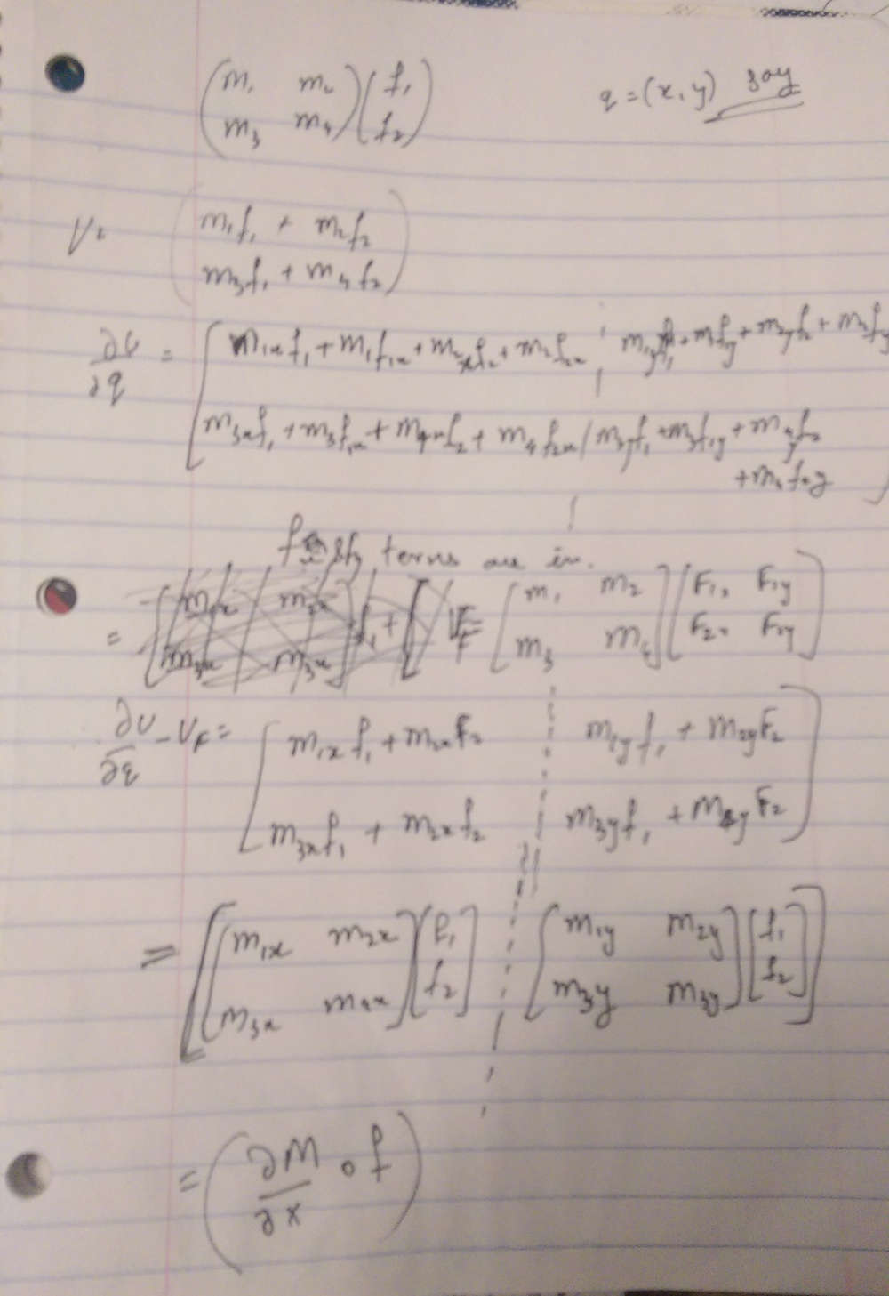
$$ \frac{\partial M(q)^{-1} }{ \partial q} = - M(q)^{-1} \frac{\partial M(q)}{\partial q} M(q)^{-1} $$Note, derivative of matrix with respect to a vector gives a tensor whose each entry is a matrix and i'th matrix is derivative of the matrix \( M(q) \) with respect to \(q_i \). \(\circ \) product of tensor with respect to a vector function gives a matrix. Detailed description/equations can be found here here
% main_derive_eom
clc
close all
clear all
addpath Screws;
addpath fcn_support;
addpath fcn_models;
define_syms;
get_kinematics_cart;
get_EOMs_cart;% define symbols to use here % cart
syms m_cart x dx ddx g 'real'
syms m_mass l th dth ddth 'real'
syms u_th 'real'

vars = {'x','th','dx','dth', ...
'm_cart','m_mass','l','u_th','g'};% get_kinematics_cart; % Position of mass 1 q = [x;th]; dq = [dx;dth];
% Position of cart
P_cart = [ x;0];

% Position of mass 2
P_mass = [ x-l*sin(th);
    l*cos(th)];

write_kin = 1;

if write_kin == 1;
    write_file(P_cart,'P_cart.m',vars); % Writing KE
    write_file(P_mass,'P_mass.m',vars); % Writing PE
end% get_EOMs_cart;
q_v = [x;
    th;];
dq_v = [dx;
    dth;];
dq = get_vel(q_v,q_v,dq_v);

% Velocity of the cart
v_cart = get_vel(P_cart,q_v,dq_v);
v_cart = simplify(v_cart);
% get_EOMs_cart (contd.)
KE_cart = 1/2*m_cart*v_cart.'*v_cart;
PE_cart = m_cart*g*P_cart(2);

% use .' because ' results in conjugate transpose.
% Velocity of the mass

v_mass = get_vel(P_mass,q_v,dq_v);
v_mass = simplify(v_mass);

KE_mass = 1/2*m_mass*v_mass.'*v_mass; % No rotational term as its point mass
PE_mass = m_mass*g*P_mass(2);

KE_total = KE_mass + KE_cart;
PE_total = PE_mass + PE_cart;
% get_EOMs_cart (contd.)
[Mr,Cr,Gr] = get_mat(KE_total,PE_total,q_v,dq_v);
U = [0;u_th];

ff = U - Cr*dq_v - Gr;


write_eom = 1;
if write_eom == 1;
    write_file(ff,'ff_cartpole.m',vars); % Writing FF
    write_file(Mr,'M_cartpole.m',vars); % Writing M

    write_file(KE_total,'KE_cartpolel.m',vars); % Writing KE
    write_file(PE_total,'PE_cartpole.m',vars); % Writing PE
endsyms x_d dx_d 'real'
syms th_d dth_d 'real'
syms u_th_d 'real'
vars_d = {'x_d','th_d','dx_d','dth_d','u_th_d', ...
'm_cart','m_mass','l','g'};
tau_d = u_th_d;
tau_v = [u_th];
X_q = [x;th; dx;dth];
X_q_d = [x_d;th_d; dx_d;dth_d];
[dfdq,dMdq,dfdu] = linearize_MF(Mr,ff,X_q,tau_v,X_q_d,tau_d);%% Linearize MF
function [dfdq,dMdq,dfdu] = linearize(M,ff,x,u,x_d,u_d)

n_states = length(x);
n_controls = length(u);

for i_s = 1:n_states/2,
    dfdq(:,i_s) = subs(diff(ff,x(i_s)) , [x;u],[x_d;u_d]);

end
for i_s = 1:n_states/2,
    dMdq(:,:,i_s) = subs(diff(M,x(i_s)) , [x],[x_d]);
end
for i_u = 1:n_controls,
    dfdu(:,i_u) =subs(diff(ff,u(i_u)) , [x;u],[x_d;u_d]);
end