Outline
- Optimal control formulation
- Linear quadratic regulator (LQR) control formulation (first variance principles)
- Dynamic programming for LQR
- Path planning
- LQR using dynamic programming
- Optimization under constraints
- Direct collocation/Direct transcription/Multiple shooting
- Bang-bang control
Recap
- State space representation
- Controllability
- Pole-placement for different control applications.
clc;close all;clear all
K_high = [100 40];K_low =[20 .8];
x0= [10;0];
t = 0:0.01:10;
K = K_high;
sys_fun = @(t,x)[x(2); -K*x];
[t X_high] = ode45(sys_fun,t,x0);
K = K_low;
sys_fun = @(t,x)[x(2); -K*x];
[t X_low] = ode45(sys_fun,t,x0);
plot(t,K_high*X_high',t,K_low*X_low')
legend('Control: High K','Control: Low K')

Optimal control
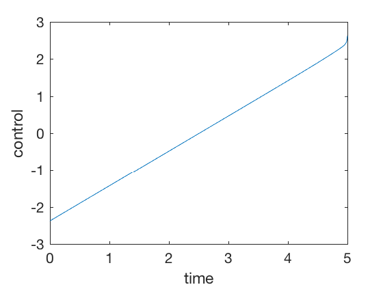
Optimal control signal that takes from point 10 to 0, is shown below. Note the magnitude of optimal control, absolute value of optimal control is less than 4. Lets look at 2 PID controls
Optimal control formulation
General case: NO time, path or control constraint.
System dynamics
$$ \dot{X} =f(x,u), $$with initial condition \( X(0) = X_0 \).
Problem statement
Define a cost function,
$$ J(u) = \Phi(X_f) + \int_{t=0}^{t_f} L(t,X,u) dt . $$Find a control policy \( u \) that minimizes,
$$ Minimize ~ J (u) $$Subject to, \( \dot{X} = f(X,u) \text{ and } \) and \( X(0) = X_0 \).
Necessary conditions
- Append system dynamics
- Define Hamiltonian \( H( x,u,\lambda ) \) as,
- Cost function changes as,
- Apply Integration by parts to last term
- Substituting it back in the integrand,
Necessary conditions (cont.)
- The integrand is,
- Taking first variance with respect to control ,
- The expression above is 0 if,
Necessary conditions for optimality (Two point boundary value problem)
Dynamic constraints: State and Costate equation
$$ \dot{\lambda}= - \frac{\partial H }{\partial X}^T , $$ $$ \dot{X} = f(X,u) \text{ and } $$Stationary conditions
$$ \frac{\partial H }{\partial u} = 0$$Boundary conditions: Initial and Final time condition
$$ \lambda_f = \left. \frac{\partial \Phi }{\partial X} ^T \right|_{t_f,X_f} . $$ $$X(0) = X_0 $$Note: \( t_f \) is assumed to be fixed. For a detailed treatment of optimal control problems under various constraints, refer to Applied Optimal Control by Bryson and Ho.
Solving necessary conditions
- States defined at initial time
- Costate defined at final time
- A diffucult 2 point boundary value problem to solve
- Both state and costate dynamic equations depend on each other.
For linear systems, we can get a state-independent representation of costate equation by expressing costate as a linear function of states and cost is a quadratic function of state and control (LQR).
Linear Quadratic Control (LQR)
In LQR we choose controller to minimize a quadratic cost of states and control,
$$ J(u) =\frac{1}{2} X_f^T S X_f +\frac{1}{2} \int_{t=0}^{t_f} (X^TQX + u^T R u) dt . $$- \( Q \) is a semi-positive definite matrix representing the cost on state deviations
- \( R \) is a positive-definite matrix indicating the control cost
- \( S \) is a positive definite matrix penalizing the error from the final desired value of \( 0 \)
\( Q \) and \( R \) define the relative weighing between control and state costs.
- For \( norm(R) >> norm(Q) \), control cost is penalized heavily, and the resulting controller drives errors to zero slower.
- For \( norm(Q) >> R \), trajectory error cost is penalized heavily, and the resulting controller drives errors to zero very quickly.
- The control corresponding to larger diagonal value of \(norm(R) \) will be used sparingly.
- The states corresponding to larger diagonal values of \(Q\) will be driven to zero faster.
Linear Quadratic Control (LQR), Necessary conditions.
Hamiltonian for LQR control is,
$$ H(X,u, \lambda) = \frac{1}{2} \left( X^TQX + u^T R u \right)+ \lambda^T (AX + Bu) $$The optimality conditions now become,
$$ \dot{\lambda}= - A^T \lambda + Q X, $$ $$ 0= B^T \lambda + R u, $$ $$ \dot{X} = AX + Bu . $$With boundary conditions \( X_0 = X(0)\) and \( \lambda_f = S X_f \).
We expect control to be a function of states, therefore, we choose \( \lambda = P X \). Substituting,
$$ \dot{P} X + P \dot{X} = - A^T PX - Q X. $$$$ \dot{P} X + P (AX + Bu) = - A^T PX - Q X. $$Using \( u = - R^{-1} B' \lambda = - R^{-1} B' P X \),
$$ \dot{P} X + P (AX - B R^{-1} B' P X) = - A^T PX - Q X. $$Rearranging gives,
$$ - \dot{P} X = A^T PX + P AX - PB R^{-1} B' P X + Q X. $$The expression above is true for all \( X \), therefore,
$$ - \dot{P} = A^T P + P A - PB R^{-1} B' P + Q . $$Equation above is called Riccati equation.
clc
close all
clear all

t_f = 10;dt = 0.001;
P_f= 100*eye(2);

Q = .0001*eye(2);R = 1;A = [0 1;0 0];B = [0 ;1];
P0 =P_f;N = t_f/dt+1;

% add t_dis array
t_dis = 0:dt:t_f;
t_res = t_f:-dt:0;

% USING ODE45 method
[t, P_all] = ode45(@(t,X)P_sys(t,X,A,B,Q,R),t_res,P0);
P_all_res_ode =   reverse_indices(P_all); % P_all is labeled with time to go.
X_ode(:,1) =[10;0];
for i = 2:length(t_dis)
    P_ode = reshape(P_all_res_ode(i-1,:),size(A));
    U_ode(:,i-1) = -inv(R)*B'*P_ode*X_ode(:,i-1);
    X_ode(:,i) = X_ode(:,i-1) + dt* (A*X_ode(:,i-1) + B*U_ode(:,i-1) );
end
plot(t_dis,X_ode);xlabel('time');ylabel('States')
legend('position','velocity')

plot(t_dis(2:end),U_ode);xlabel('time');ylabel('Control')

%%% Function
function dPdt = mRiccati(t, P, A, B, Q,R)

P = reshape(P , size(A)); %Convert from "n^2"-by-1 to "n"-by-"n"
dPdt = -(A'*P + P*A - P*B*B'*P + Q); %Determine derivative
dPdt = dPdt(:); %Convert from "n"-by-"n" to "n^2"-by-1

%%% Function
function P_rev = reverse_indices(P)
for  i = 1:size(P,1)
   P_rev(i,:) = P(size(P,1)-i+1,:);
end
Practical considerations
- Initialize \( Q \) as very small value if we want to have \( Q = 0\).
- Backwards time calculation is expensive
- Save the solution of the time-dependent Riccati equation indexed by the time to go.
- This scheme works only for linear systems.
- To apply this scheme for linearized systems, the P matrix has to be computed as each time-step because the
- For large finite time, finite and infinite time LQR are equivalent
Continuous time infinite horizon, Linear quadratic regulator
The cost function when time allowed to go to \( \infty \).
$$ J(u) = \frac{1}{2} \int_{t=0}^{\infty} (X^TQX + u^T R u) dt . $$In steady state condition, \( \dot{P} = 0 \). Therefore, the Riccati equation becomes,
$$ 0 = PA + A^T P - PB R^{-1}B^T P + Q X. $$Equation above is called Algebraic Riccati equation.
K_high = [100 40];
K_low = [40 .8];
x0= [10;0];


M_a = rank(ctrb(A,B));
t = 0:0.01:10;

P = care(A,B,Q,R);
K = inv(R)*B'*P;
K_opt = K
sys_fun = @(t,x)[x(2); -K_opt*x];
[t X_opt] = ode45(sys_fun,t,x0);

K = K_high;
sys_fun = @(t,x)[x(2); -K_high*x];
[t X_high] = ode45(sys_fun,t,x0);

K = K_low;
sys_fun = @(t,x)[x(2); -K_low*x];
[t X_low] = ode45(sys_fun,t,x0);
figure;
plot(t,X_high(:,1),t,X_low(:,1),t,X_opt(:,1),t_dis,X_ode(1,:))
legend('Position: High K','Position: Low K','Position: Opt K','Position: Fixed time')

figure;
plot(t,-K_high*X_high',t,-K_low*X_low',t,-K_opt*X_opt',t_dis(1:end-1),U_ode)
%legend('Control: High K','Control: Low K','Control: Opt K','Position: Fixed time')

Discrete time LQR control
System dynamics:
$$ X[k+1] = f(x[k],u[k]) $$Find \( u[k] \) that minimizes,
$$ J(u) =\frac{1}{2} X_f^T S_f X_f +\frac{1}{2} \sum_{k=1}^{N} (X[k]^TQX[k] + u[k]^T R u[k]). $$Initial condition \( X[1] = X_0 .\)
Expressing costate as,
$$ \lambda[k] = P[k] X[k] $$Costate at \( k+1 \) is
$$ \lambda[k+1] = P[k+1] X[k+1] = P[k+1] (A X[k] + B u[k]) $$ $$ \lambda[k+1] = P[k+1] \left( A X[k] - BR^{-1} B' \lambda[k+1] \right) $$Rearranging,
$$ \left(I + P[k+1]BR^{-1} B' \right) \lambda[k+1] = P[k+1] A X[k]$$ $$ \lambda[k+1] = \left(I + P[k+1]BR^{-1} B' \right)^{-1} P[k+1] A X[k]$$Control can be written as,
$$ u[k] = -R^{-1} B^T \lambda[k+1] = -R^{-1} B^T \left(I + P[k+1]BR^{-1} B' \right)^{-1} P[k+1] A X[k]$$Costate propogation,
$$ \lambda[k] = A^T \lambda[k+1] + Q X[k] $$ $$ P[k] X[k] = A^T \left(I + P[k+1]BR^{-1} B' \right)^{-1} P[k+1] A X[k] + Q X[k] $$As above equation is satisfied for all \( X[k] \), we get
$$ P[k] = A^T \left(I + P[k+1]BR^{-1} B' \right)^{-1} P[k+1] A + Q $$Equation above is called Riccati equation. For discrete time, Riccati equation is more complex, and comes in different forms based on how it is derived.
Different forms of Riccati equations
Form 1 $$ P[k] = A^T (I + P[k+1] B R^{-1} B^T)^{-1}P[k+1] A + Q $$
Form 2
$$ P[k] = A^T P[k+1] A - A^T P[k+1] B (R + B^T P[k+1]B )^{-1} B^T P[k+1]A + Q $$Discrete time LQR control: Necessary conditions
At infinite time, \( P[k] = P[k+1] \), therefore, the optimality conditions change as,
$$ P = A^T P A - A^T P B (R + B^T P B )^{-1} B^T P A + Q $$This expression is called Algebraic Riccati equation, and can be solved using MATLAB's 'dare' command.
clc
close all
clear all

t_f = 4;
dt = 0.02;
t_dis = 0:dt:t_f;
N = length(t_dis);
S{N} = 100*eye(2);
R = dt;Q = .0001*eye(2)*dt;A = [1 dt;0 1];B = [0 ;dt];
for i = N-1:-1:1

    K{i} = inv(R + B'*S{i+1}*B)*B'*S{i+1}*A;
    %S{i} = Q + K{i}'*R*K{i} + (A-B*K{i})'*S{i+1}*(A-B*K{i}); % First form
    S{i} = Q+ A'*S{i+1}*A - A'*S{i+1}*B*inv(R+B'*S{i+1}*B)*B'*S{i+1}*A;% Second form
    %S{i} =  A'*inv(eye(2) + S{i+1}*B*inv(R)*B')*S{i+1}*A + Q; % Third form


end
X(:,1) = [10;0];
X_dlqr(:,1) = [10;0];
P_dlqr = dare(A,B,Q,R);
K_dlqr = inv(R)*B'*P_dlqr;
for i = 1:N-1
    u(i) = -K{i}*X(:,i);
    X(:,i+1) = A * X(:,i) + B*u(i);
    X_dlqr(:,i+1) = A * X_dlqr(:,i) - B*K_dlqr*X_dlqr(:,i) ;
end
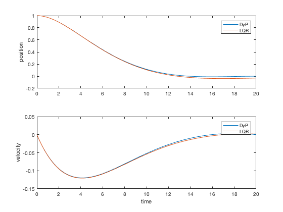
figure;
subplot(2,1,1)
plot(t_dis,X(1,:),t_dis,X_dlqr(1,:))
legend('Finite time LQR','Infinite time LQR')
ylabel('position')
subplot(2,1,2)
plot(t_dis,X(2,:),t_dis,X_dlqr(2,:))
ylabel('velocity')
xlabel('time')

LQR limitations
- Not all cost functions can be expressed as LQR problem. Consider the case when we are trying to minimize the time to go.
- LQR formulations do not generalize well to conditions when additional constraints are imposed on the system.
- For control inequality constraints, the solution to LQR applies with the resulting control truncated at limit values.
- Dealing with state- or state-control (mixed) constraints is more difficult, and the resulting conditions of optimality are very complex. See Applied optimal control, by Bryson and Ho for detailed treatment.
In the cases above, numerical methods are more suitable.
Dynamic programming
- LQR conditions very difficult to solve.
- Dynamic programming is a very powerful and versatile method to solve optimization problems
- Examples include, path planning, generating shortest cost path between cities, inventory scheduling, optimal control, rondevous problems and many more.
Dynamic programming introduction
- Define a cost-to-go function at each state value. Once this cost-to-go map is available
- Optimal control policy can be obtained by moving from one state to another state that minimizes the cost to go from that state
- Solve for control backwards starting from final conditions
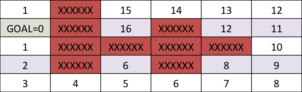
Simple example: Dynamic programming
Find the shortest path between the target and and any start position on the grid

One step back
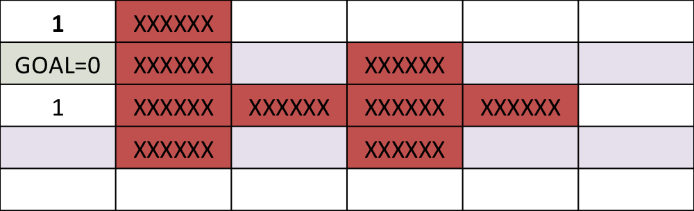
5 steps back
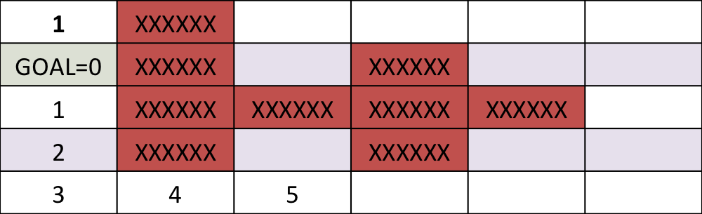
Final cost-to-go map
Dynamic programming: Algorithm 1
- Initialization
- Set cost-to-go, J to a large value.
- Discretize state-action pairs
- Set cost-to-go as 0 for the goal.
- Set point_to_check_array to contain goal.
- Repeat until elements in point_to_check_array = 0
- For point element in point_to_check_array
- Step backwards from point, and compute cost of taking action to move to the point as cost-to-go from point plus the action cost.
- If current cost-to-go, J is larger than the cost-to-go from point to moved state, then update cost-to-go for the moved state.
- Add moved state to a new point_to_check_array
- For point element in point_to_check_array
Dynamic programming: Algorithm 2
- Initialization
- Set cost-to-go, J to a large value.
- Discretize state-action pairs
- Set cost-to-go as 0 for the goal.
- Set point_to_check_array to contain goal.
- Repeat until no-values are updated,
- For each element in the grid, take all the possible actions and compute the incurred costs.
- For each action, compute the cost-to-go of the new state.
- Update self if cost-to-go of the new state plus action is lower than current cost-to-go.
Dynamic programming: Cost-to-go
Cost-go-approximation
$$ J(x[k]) = \underbrace{min}_{u[k]} \left[ L(x[k] , u[k], x[k+1]) + J(x[k+1]) \right]$$V = Act;
gam = .9;
for i_Q = 1:1000
for i_x = 2:length(x)-1
for i_y = 2:length(y)-1
iv_x = [1 0 -1 1 0 -1 1 0 -1];
iv_y = [1 1 1 0 0 0 -1 -1 -1];
for i_v = 1:9,
d =sqrt( (iv_x(i_v))^2 + (iv_y(i_v))^2 );
Va(i_v) = V(i_x+iv_x(i_v),i_y+iv_y(i_v));
Rew(i_v) = -d + Act(i_x+iv_x(i_v),i_y+iv_y(i_v));
end
[V_max , i_vmax]= max(Va);
V_new(i_x,i_y) = gam*V_max + Rew(i_vmax);
if V(i_x,i_y) == -100,
V_new(i_x,i_y) = V(i_x,i_y);
end
end
end
V = V_new;
end
MATLAB demo
Dynamic programming in control vs reinforcement learning.
The same ideas of dynamic programming can be applied in reinforcement learning also.
- In reinforcement learning the objective is to maximize reward
- In control theory objective is to minimize cost.
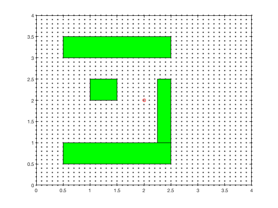
Reinforcement learning: Value function
Reinforcement learning: Obstacle avoidance
Dynamic programming for LQR
We will next apply the procedure above to compute optimal control for a linear system given by,
$$ X[k] = A X[k-1] + B u[k-1]$$Consider designing a controller for the
$$ J(x[k]) = \underbrace{min}_{u[k]} \left[ \frac{1}{2}\left( X[k]^TQX[k] +u[k]^TRu[k] \right) + J(x[k+1]) \right] $$with
$$ J(x[N]) = \frac{1}{2} X[N]^T S_NX[N] ,$$being the cost at the end of the cycle. We start the dynamic programming by stepping backwards from \( N \)
$$ J(x[N-1] ) = \underbrace{min}_{u[N-1]} \left[ \frac{1}{2}\left( X[N-1]^TQX[N-1] +u[N-1]^TRu[N-1] \right) + J(x[N] ) \right] $$Cost at final time
$$ J(x[N] ) = \frac{1}{2} X[N]^TS_NX[N] ,$$ $$ J(x[N] ]) = \frac{1}{2} \left( A X[N-1] + Bu[N-1] \right)^TS_N(A X[N-1] + Bu[N-1]) ,$$Substituting in Bellman equation
$$ J(x[N-1] ) = \underbrace{min}_{u[N-1]} \left[ \frac{1}{2}\left( X[N-1]^TQX[N-1] +u[N-1]^TRu[N-1] \right) + \frac{1}{2} (A X[N-1] + Bu[N-1])^TS_N(A X[N-1] + Bu[N-1]) \right] $$Taking derivative w.r.t \( u[K-1] \)
$$ \frac{\partial J(x[N-1] )}{\partial u[N-1]} = \left[ u[N-1]^T R + (A X[N-1] + Bu[N-1])^T S_N B \right] = 0 $$As \( R \) and \( S_N \) are symmetric,
$$ R u[N-1] + B^T S_N (A X[N-1] + Bu[N-1]) = 0 $$ $$ u[N-1] = - (R+ B^T S_N B)^{-1} B^T S_N A X[N-1]$$Defining K as
$$ K_{N-1} = (R+ B^T S_N B)^{-1} B^T S_N A X[N-1]$$ $$ J(x[N-1] ) = \left[ \frac{1}{2}\left( X[N-1]^TQX[N-1] +u[N-1]^TRu[N-1] \right) + J(x[N] ) \right] $$ $$ J(x[N-1] ) =\frac{1}{2} \left[ \left( X[N-1]^TQX[N-1] +X[N-1]^T K_{N-1}^T R K_{N-1} u[N-1] \right) + X[N-1]^T(A - B K_{N-1} )^TS_N(A - B K_{N-1} X[N-1] ) \right] $$Redefining S as
$$ S_{N-1} = Q+ K_{N-1}^T R K_{N-1} + (A - B K_{N-1} )^TS_N(A - B K_{N-1}) $$\( J(x[N-2] ) \) becomes
$$ J(x[N-2] ) = \frac{1}{2} \underbrace{min}_{u[N-2]} \left[ \left( X[N-2]^TQX[N-2] +u[N-2]^TRu[N-2] \right) + J(x[N-1] \right] $$with
$$ J(x[N-1] ) = \frac{1}{2} X[N-1]^T S_{N-1} X[N-1] ,$$Riccati equation
$$ S_{N-1} = Q+ K_{N-1}^T R K_{N-1} + (A - B K_{N-1} )^TS_N(A - B K_{N-1}) $$with
$$ K_{N-1} = (R+ B^T S_N B)^{-1} B^T S_N A X[N-1]$$Numerical methods for optimal control: Shooting methods
- LQR formulation cannot handle state or control constraints.
- Bound constraints on control result in the same control law, with control truncated at limits.
- For other cases, the first variance methods result in complex equations
- Numerical methods can be used to solve complex problems
Shooting methods used to compute optimal control laws.
Shooting method
Assume control and state trajectory. Integrate dynamics equations using control, and minimize the error between this trajectory and assumed polynomial state trajectory.
- Direct methods: Approximate control and state by polynomials,and minimize the error between dynamics and future points using nonlinear programming.
- Indirect methods: Derive optimiality conditions, and find solutions that satisfy these conditions at a few intermediate points.
Problem formulation
Find control sequence to minimize,
$$ J(u) = \Phi(X_f) + \int_{t=0}^{t_f} L(t,X,u) dt . $$Subject to,
$$ \dot{X} =f(x,u), $$with initial condition \( X(0) = X_0 \), under constraints,
$$ u_{min} \leq u \leq u_{max}, $$ $$ X_{min} \leq X \leq X_{max}, $$ $$ C_{eq}(X,u) = 0 , $$ $$ C(X,u) \leq 0 , $$where \( C_{eq} \) and \( C \) are equality and inequality constraints
Parametarization of optimial control using polynomial functions
Express states and control as a piece-wise continuous function of time,
$$ q_{i,i+1}(t) = p_q(t) $$$$ u_{i,i+1}(t) = p_u(t) $$Parameterize control and state by knot points, \( u_i \) and \( q_i \) for \( i \) going from \( 1 to N+1 \). Find control sequence to minimize,
$$ J \left( i: 1 \rightarrow N, u_{i,i+1},q_{i,i+1}) \right) = \Phi_p(q_f) + \sum_{i=1}^N L_p(u_{i,i+1},q_{i,i+1}) . $$Subject to,
$$ q_{i+1} = \int_{t=t_i}^{t_{i+1}}f(x,u)dt, $$Find control sequence to minimize,
$$ J \left( i: 1 \rightarrow N, u_{i,i+1},q_{i,i+1}) \right) = \Phi_p(q_f) + \sum_{i=1}^N L_p(u_{i,i+1},q_{i,i+1}) . $$Subject to,
$$ q_{i+1} = \int_{t=t_i}^{t_{i+1}}f(x,u)dt, $$Initial condition \( X(i) = q_i .\)
with control
$$ u_{i,i+1}(t) $$under constraints,
$$ u_{min} \leq u_i \leq u_{max}, $$ $$ X_{min} \leq q_i \leq X_{max}, $$ $$ C_{p,eq}(q_i,u_i) = 0 , $$ $$ C_p(q_i,u_i)\leq 0 . $$Nonlinear programming: quick review
As state above, we convert optimal control problem into a simpler task of identifying the knot-points, coefficient of polynomials or other parameters that define a state/control trajectory. This is a parameter optimization problem, and is much simpler than solving LQR equations. Say we want to minimize \( f(X) \), such that,
$$ A X \leq B , \text{ inequality constraint}$$$$ A_{eq} X = B_{eq} , \text{ equality constraint}$$$$ C(X) \leq 0 , \text{ inequality non-linear constraint}$$$$ C_{eq}(X) = 0 , \text{ equality non-linear constraint}$$$$ X_l \leq X \leq X_u. \text{Bounds} $$Such problems can be solved using nonlinear solvers, such as fmincon.
$$x = fmincon(fun,x0,A,b,Aeq,beq,lb,ub,nonlcon,options)$$Fmincon: example 1
$$ J(X_1,X_2) = 100(X_2^2 -X_1)^2 + (1-X_1)^2 $$Subject to the constraint that,
$$ 2X_1+X_2 = 1 $$fun = @(x)100*(x(2)-x(1)^2)^2 + (1-x(1))^2;
x0 = [0.5,0];
A = [1,2];
b = 1;
Aeq = [2,1];
beq = 1;
x = fmincon(fun,x0,A,b,Aeq,beq)
Fmincon: Canon example
Consider the example of firing a cannon such that the cannonball reaches a particular target while requiring minimum firing energy. The equations of motion describing the movement of cannon ball are given by,
$$x(t) = v_x t $$ $$y(t) = v_y t - \frac{1}{2}gt^2 $$The objective of optimization is given by,
$$ \underbrace{Minimize}_{v_x,v_y} (v_x^2+v_y^2)$$The boundary conditions are given by,
$$ x(t_f) = 10, y(t_f) = 0 $$$$ t_f \geq 0.001 $$$$ v_x \geq 0 $$$$ v_y \geq 0 $$$$ x(t_f) = 10 $$$$ y(t_f) = 10 $$clc
close all
clear all
N_grid = 10;
t_f =3;
v_x = 4;
v_y = 10;
X0 = [t_f;v_x;v_y];
X_opt = fmincon(@(X)cost_fun_cannon(X),X0,[],...
[],[],[],[],[],@(X)cons_fun_cannon(X),options);
%%% Cost function
function cost= cost_fun_cannon(X)
N_grid = (length(X)-3)/3;
% Cost fun
t_f = X(1);
vx = X(2);
vy = X(3);

cost = vx^2+vy^2;

%%% Constraint function
function [C,Ceq] = cons_fun_cannon(X)
N_grid = (length(X)-3)/3;
t_f = X(1);
vx = X(2);
vy = X(3);
d_x = t_f*vx;
d_y = vy*t_f -1/2*9.8*t_f^2;

C = [-t_f+0.001;
    -vx;
    -vy];
Ceq = [d_y-10;
            d_x - 10;
];
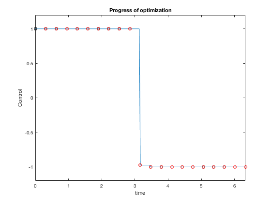
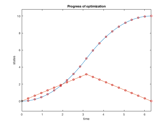
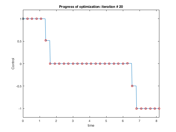
Bang-bang control
Given \( \ddot{X} = u \) find minimum time trajectory given \( -1 \leq u \leq 1 \).
$$ minimize (t_f)$$given,
$$ -1 \leq u \leq 1$$ $$ X_0 = 10, X_f = 0. $$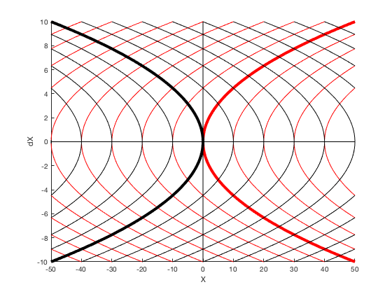
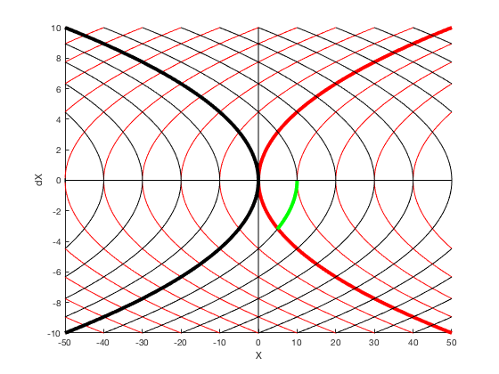
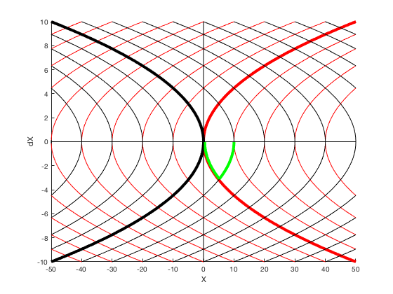
Solution process
- Express control as a piece-wise constant function
- The position and velocity variables defined at the knot points form the additional input to the optimizer
- Integrate the states starting with one knot point to another assuming approximate control and apply equality constraints
function [C,Ceq] = cons_fun_doubleIntegrator(X,type)
% Assuming cosntant U
N_grid = (length(X)-1)/3;
% Cost fun
t_f = X(1);
X1 = X(2:N_grid+1);
X2 = X(2+N_grid:2*N_grid+1);
u = X(2+2*N_grid:3*N_grid+1);
C = [];
Ceq = [X2(1) - 0;
    X2(end) + 0;
    X1(1);
    X1(end)-10;
    ];
time_points = (0:1/(N_grid-1):1)*t_f;
for i = 1:(N_grid-1)
    X_0(1,:) = X1(i);    X_0(2,:) = X2(i);
    t_start = time_points(i);t_end = time_points(i+1);

    tt = t_start:(t_end-t_start)/10:t_end;

    [t,sol_int] = ode45(@(t,y)sys_dyn_doubleIntegrator(t,y,X,type),tt,X_0);
    X_end = sol_int(end,:);

    Ceq = [Ceq;
        X_end(1) - X1(i+1);
        X_end(2) - X2(i+1)]; % IMPOSING DYNAMIC CONSTRAINTS AT BOUNDARIES.
end
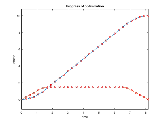
Bang-bang control: Example 2
Now we impose additional constraint that the velocity cannot go above 1.5. The problem changes as, given the double integrator system \( \ddot{X} = u \),
$$ minimize (t_f)$$given,
$$ -1 \leq u \leq 1$$ $$ \dot{X} \leq 1.5 $$ $$ X_0 = 10, X_f = 0. $$function [C,Ceq] = cons_fun_doubleIntegrator(X,type)
% Assuming cosntant U
N_grid = (length(X)-1)/3;
% Cost fun
t_f = X(1);
X1 = X(2:N_grid+1);
X2 = X(2+N_grid:2*N_grid+1);
u = X(2+2*N_grid:3*N_grid+1);
C = [X2-1.5];
Ceq = [X2(1) - 0;
X2(end) + 0;
X1(1);
X1(end)-10;
];
time_points = (0:1/(N_grid-1):1)*t_f;
for i = 1:(N_grid-1)
X_0(1,:) = X1(i); X_0(2,:) = X2(i);
t_start = time_points(i);t_end = time_points(i+1);
tt = t_start:(t_end-t_start)/10:t_end;
[t,sol_int] = ode45(@(t,y)sys_dyn_doubleIntegrator(t,y,X,type),tt,X_0);
X_end = sol_int(end,:);
Ceq = [Ceq;
X_end(1) - X1(i+1);
X_end(2) - X2(i+1)]; % IMPOSING DYNAMIC CONSTRAINTS AT BOUNDARIES.
end
Practical guidelines for desgining optimization routines
- Initialization is very crucial. Its good to initialize states and velocities as linear functions, and control as 0.
- The resulting control policy satisfies constraints and dynamic equations only at the knot points. Therefore, to ensure safety have a safety margin within the limits, so intermediate points do not violate boundary constraints.
- In cases where you know the form of control equation (polynomial, piecewise constant), use it to inform the optimizer.
- Optimality (lowest cost solution) can be improved by either changing the number of grid points or order of polynomials. However, systems with more parameters have larger
- Start with a simpler low-dimensional polynomial on a coarser grid and use this to inform an optimizer with more parameters.