Motivation
- Transform an original n-order nonlinear control system into a first order sytem.
- Simplify the original dynamics so control design becomes easier.
- Force the system dynamics onto a manifold such that the resulting dynamics becomes simple.
Motivation,
Given a n-order system, \( X^{(n)} = f(X) + g(X) u \), transform it into a first order dynamics using a variable \( s \). \( s \) satisfies the following 2 properties,
- \( \dot{x} \) contains \( u \).
- If \( s \rightarrow 0 \) then \( x \rightarrow 0 \).
Choose control such that \( s = 0 \) once the states reach sliding manifold.
Example Sliding mode:
For \( n = 2 \), say a system is given by,
$$ \ddot{x} = f(x) + g(x)u $$We wish to drive \( x \rightarrow x_d \) and \( \dot{x} \rightarrow \dot{x}_d \). Choose \( s \) such that
- \( \dot{x} \) contains \( u \).
- If \( s \rightarrow 0 \) then \( x \rightarrow 0 \).
Choose
$$ s = \lambda (x - x_d ) + ( \dot{x} - \dot{x}_d)=\lambda e+ \dot{e}$$For a general \( n \) order system, the sliding variable can be selected as,
$$ s = \left( \frac{d}{dt} + \lambda \right)^{n-1} e $$Note in the expressions above, \( e \) can be considered as a filter response to input \( s \), therefore if \( s \rightarrow 0 \), then \( x \rightarrow 0 \).
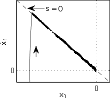
Geometric interpretation
- For 2-dimension case, \( s = \dot{e} + \lambda e\) represents a line with slope of \( -\lambda \) in the phasephot, and the line contrains origin.
- In general, if we plot \( x \) vs \( \dot{x}\), then the line will pass through \( x_d \) and \( \dot{x}_d \) and will have the slope of \( -\lambda\).
For a general n-dimension system, \( s= 0\) represents a hyperplane in the \( n-1 \) that passes through the origin (or desired point) depending on the variable representation.
Boundedness of states
Say we are able to bound the sliding variables \( s \) such that \( |s|\leq \phi \) after some transient dynamics. We are interested in the bounds on the error \( e \) when \(|s| \leq \phi \). We will consider a second order system first, in this case, the sliding variable is given by,
$$ s = \dot{e} + \lambda e $$ $$ \lambda exp(\lambda t) e + exp(\lambda t) \frac{de}{dt} = exp(\lambda t) s $$$$ \frac{d(exp(\lambda t)e)}{dt} = exp(\lambda t) s $$$$ d(exp(\lambda t)e) = exp(\lambda t) s dt $$Integrating between \( t_f \) and \( 0 \) gives,
$$e(T) = e(0) exp(-\lambda T) + \int_0^T exp(-\lambda (T-t)) s dt $$We will study the boundedness of \( e(T) \) as \( T \rightarrow \infty \). As \( T \) becomes large, \( exp(-\lambda T) \rightarrow 0 \), for \( \lambda >0 \). Therefore, the first term is bounded, we will investigate the second term only. As \(|s| \leq \phi \),
$$ \int_0^T exp(-\lambda (T-t)) s dt \leq \phi \int_0^T exp(-\lambda (T-t)) dt$$Integrating the term on the right gives,
$$ \frac{\phi}{\lambda} (1-exp(-\lambda T)) \leq \frac{\phi}{\lambda} $$Therefore, the error \( e \) is bounded by \( \phi/\lambda \). We can show that for a n-dimension system, the error is bounded by,
$$ e \leq \frac{\phi}{\lambda^{n-1}} $$Therefore, if we are able design a control that ensures \( s \leq \phi \) we are assued due to sliding variable that \( e \leq \frac{\phi}{\lambda^{n-1}} \).
Sliding mode control:
Say we are intersted in controlling a second order system given by,
$$ \ddot{x} = f(x,\dot{x}) + g(x,\dot{x}) u $$Once we design the sliding variable, we can design control based to drive \( s \rightarrow 0 \). Define a Lyapunov function \( L \) as,
$$ L = \frac{1}{2}s^2 $$Taking derivative gives,
$$ \dot{L} = s \dot{s} $$Therefore, if we choose \( u \) such that \( s \dot{s} < 0 \) always, then the \( s \rightarrow 0 \). The derivative of Lyapunov can we written as,
$$ \dot{L} = s ( \ddot{x} + \lambda \dot{x}) = s ( f(x,\dot{x}) + g(x,\dot{x}) u + \lambda \dot{x})$$choosing \( u = - g(x,\dot{x})^{-1} (f(x,\dot{x}) + \lambda \dot{x} + \eta sign(s))\)
$$ \dot{L} = - \eta |s| $$- The resultant control is chosen as \( \eta sign(s) \) instead of \( -\eta s \) to have a constant 'velocity' towards the sliding surface.
- This ensures that we reach the sliding surface in a finite time and not asymptotically.
Example 1 :
Consider the example of a system given by,
$$ \ddot{x} + 1.5 \dot{x}^2cos(3x) = u $$with \( 1 \leq a(t) \leq 2 \), we would like to convert this to a first order system. Lets define a sliding variable \( s\),
$$ s = \dot{x} + \lambda x $$as \( x \) is a first order response to \( s \). \(s \) satisfies,
- \( x \rightarrow 0 \) as \( s \rightarrow 0 \)
- \( \dot{s} \) contains \( u \)
Therefore, \( s \) is a valid choice for sliding variable.
Choose the Lyapunov, \( L \) as
$$ L = \frac{1}{2} s^2 $$Taking derivative of \( L \) gives,
$$ \dot{L} = s \dot{s} =s ( \ddot{x} + \lambda \dot{x}) = s (u - 1.5 \dot{x}^2cos(3x)) + \lambda x $$Choosing \( u = 1.5 \dot{x}^2cos(3x)) - \lambda x - \eta sign(s) \). gives,
$$ \dot{L} = - \eta |s|$$clc
close all
clear all
x(:,1) = [1;1];
dt = 0.01;
lambda = 1;
eta = 5;
for i = 2:2000,
s(i) = x(2,i-1)+lambda*x(1,i-1);
u(i) = 1.5*x(2,i-1)^2*cos(3*x(1,i-1)) - lambda*x(1,i-1) - eta*sign(s(i));
x(1,i) = x(1,i-1) + dt*(x(2,i-1));
x(2,i) = x(2,i-1) + dt*(u(i) - 1.5*cos(3*x(1,i-1)));
end
plot(x(1,:),x(2,:))
hold on
plot([-2:.01:2],-lambda*[-2:.01:2])
xlabel('x')
ylabel('dx/dt')

Sliding mode control for control under uncertainty:
Conside the second order true system system that is given by
$$ \ddot{x} = f(x,\dot{x}) + g(x,\dot{x}) u $$and say the approximate system we know is given by,
$$ \ddot{x} = \hat{f}(x,\dot{x}) + g(x,\dot{x}) u $$such that \( |f - \hat{f}| \leq F \). Sliding mode control lends itself very well to such problems. The technique to design control is similar. We first choose a sliding variable, \( s = \dot{x} + \lambda x \). Similar to process above, we define a Lyapunov,
$$ L = \frac{1}{2} s^2 $$Taking derivative gives,
$$ \dot{L} = s \dot{s} = s(f(x,\dot{x}) + g(x,\dot{x}) u + \lambda \dot{x}) $$Now, we do not know \( f(x,\dot{x}) \) accurately, so we can use estimate of \( f \) for designing control instead of the true \( f (x,\dot{x})\). Choosing \( u = - g(x,\dot{x})^{-1} ( \ \hat{f}(x,\dot{x}) +F + \lambda \dot{x} + \eta sign(s) )\) gives,
$$ \dot{L} = s(f(x,\dot{x}) -\hat{f}(x,\dot{x}) -F - \eta sign(s)) $$As \( |f - \hat{f}| \leq F \),
$$ \dot{L} \leq s( - \eta sign(s)) $$Therefore, the choice of control \( u = - g(x,\dot{x})^{-1} ( \ \hat{f}(x,\dot{x}) +F + \lambda \dot{x} + \eta sign(s) )\) drives \( s \rightarrow 0 \).
Example 2:
Consider the example of a system given by,
$$ \ddot{x} + a(t) \dot{x}^2cos(3x) = u $$with \( 1 \leq a(t) \leq 2 \), we would like to control this sytem so \( x \rightarrow 0 \). As we do not know \( a(t) \) precisely, we choose an estimate as, \( 1.5 \dot{x}^2cos(3x) \). Therefore,
$$ f - \hat{f} = (a(t)-1.5) x^2 cos(3x) \leq .5x^2|cos(3x)|$$We will now define a sliding variable, \( s \) as,
$$ s = \dot{x} + \lambda x $$$$ L = \frac{1}{2} s^2 $$Taking derivative of Lyapunov,
$$ \dot{L} = s (\ddot{x} + \lambda \dot{x} )= s((u - a(t) \dot{x}^2cos(3x)) + \lambda x ) $$As we do not know \( a(t) \) precisely, we can replace it with an estimate, \( 1.5 \dot{x}^2cos(3x) \)
Therefore, choosing \( u = 1.5 \dot{x}^2 cos(3x) - .5x^2|cos(3x)|- \lambda x - \eta sign(s) \) gives,
$$ \dot{L} = s( (1.5 - a(t) ) \dot{x}^2cos(3x)- .5x^2|cos(3x)| - \eta sign(s) ) $$$$\dot{L} \leq s( - \eta sign(s) ) \leq \eta |s| $$clc
close all
clear all
x(:,1) = [1;1];
dt = 0.01;
lambda = 1;
eta = 5;
for i = 2:2000,
s(i) = x(2,i-1)+lambda*x(1,i-1);
u(i) = 1.5*x(2,i-1)^2*cos(3*x(1,i-1)) - lambda*x(1,i-1) - eta*sign(s(i));
x(1,i) = x(1,i-1) + dt*(x(2,i-1));
a = 1+rand;
x(2,i) = x(2,i-1) + dt*(u(i) - a*cos(3*x(1,i-1)));
end
plot(x(1,:),x(2,:))
hold on
plot([-2:.01:2],-lambda*[-2:.01:2])
xlabel('x')
ylabel('dx/dt')

Chattering in sliding mode control:
- The sliding mode control is a discountinuous control, because we are making sure we always go towards the sliding surface with constant velocity.
This can result in chattering, when the control switches quickly around the sliding surface.
Chattering can be avoided by including a smoother transition across zero, by using a sigmoid (tanh) type of function, however, this results in a scenario where the controller may not drive the sliding variable to zero precisely, but to a neighborhood of zero.
x = -1:.01:1;
plot(x,tanh(20*x),x,sign(x))
xlabel('x')
ylabel('tanh(x)')
axis([-1 1 -1.1 1.1])

clc
close all
clear all

x(:,1) = [1;1];
dt = 0.01;
lambda = 1;
eta = 5;

for i = 2:2000,
    s(i) = x(2,i-1)+lambda*x(1,i-1);
    u(i) = 1.5*x(2,i-1)^2*cos(3*x(1,i-1)) - lambda*x(1,i-1) - eta*tanh(20*s(i));
    x(1,i) = x(1,i-1) + dt*(x(2,i-1));
    a = 1+rand;
    x(2,i) = x(2,i-1) + dt*(u(i) - a*cos(3*x(1,i-1)));

end
plot(x(1,:),x(2,:))
hold on
plot([-2:.01:2],-lambda*[-2:.01:2])
xlabel('x')
ylabel('dx/dt')
