Control and estimation under uncertainity:

MEC 560: Advaced control systems

Vivek Yadav

Recap

• State space representation
• Controllability and Pole-placement for different control applications
• Optimal control formulation
• Linear quadratic regulator (LQR) control formulation (first variance principles)
• Dynamic programming for LQR
  • Path planning
  • LQR using dynamic programming
• Multiple shooting
• Direct collocation
• Observer design

All techniques above assume a perfect model of the system.

Types of uncertainities

1. Parametric uncertainity
2. Actuator uncertainity
3. Modeling uncertainity
4. Measurement uncertainity

All the uncertainities can result in erroneous control calculation and undesired system behavior.

1. Parametric uncertainity

Uncertainity where model parameters are not accurately known.

Approximate system:

$$ \dot{X} = AX + Bu $$

with measurements

$$ Y = CX. $$

Actual system:

$$ \dot{X} = (A+ \Delta A) X + (B + \Delta B) u $$

with measurements,

$$ y = (C+ \Delta C) X $$

2. Actuator uncertainity

Uncertainity where there is error between commanded and applied control to the system

Approximate system:

$$ \dot{X} = AX + Bu $$

with measurements

$$ Y = CX. $$

Actual system:

$$ \dot{X} = A X + B ( u + \delta u) $$

with measurements, $$ y =C X$$

3. Modeling uncertainity

• Uncertainity where one or other phenomena was completely ignored.
• Linearization errors
• Dynamics change due to wear and tear, added load etc.

Approximate system:

$$ \dot{X} = AX + Bu $$

with measurements

$$ Y = CX. $$

Actual system:

$$ \dot{X} = A X + B u + f(X,u) $$

with measurements,

$$ y =C X +g(X,u) $$

4. Measurement uncertainity

• Measurements have errors due to noise in the sensor

Approximate system:

$$ \dot{X} = AX + Bu $$

with measurements

$$ Y = CX. $$

Actual system:

$$ \dot{X} = A X + B u $$

with measurements, $$ y =C X + \nu $$

Control/estimation under uncertainity: Two approaches

1. Model uncertainity as gaussian process

• Kalman filter
• LQG control

2. Choose control to minimize sesitivity to errors.

• H2 control
• H-\( \infty \) control

Kalman filter

• Also called Linear Quadratic Estimator, is observability equivalent of Linear Quadratic Regulator.
• Find the states that satisfy the system dyanmics and measurement
• Originally posed as a least-square problem, to minimize difference between state estimates and measurement, while satisfying system dynamics.
• Assumes Gaussian distribution, optimal ONLY if the underlying distribution is Gaussian.
• Updated based on Bayes' rule.

Kalman filter: Main idea

• Estimate future states based on system dynamics
• Update state estimates after getting measurement
• Find gain that minimizes error between true expected state and estimated state.

Bayesian inference

Bayesian inference is based on Bayes theorem, and gives probability of an event based on features that may be related to an event.

• Bayes' rule

$$ P(A|B) = \frac{P(B|A) P(A)}{P(B)}. $$

• Another form

$$ P(A|B) = \frac{P(B|A) P(A)}{P(B|A) P(A) + P(B| \neg A) P(\neg A)} , $$

• If the event \( A \) can take multiple values say \( A_i \) for \( i : 1 \rightarrow N \).

$$ P(A|B) = \frac{P(B|A) P(A)}{ \sum_{i=1}^N P(B|A_i) P(A_i) } , $$

Example 1: Cancer testing

Say we have a test for cancer that is 99% accurate, i.e. given a person has cancer, the test gives a positive test 99% of the time. This is also referred as the true-positive rate or sensitivity. Further, if a person does not have cancer, the test gives a negative result 98% of the time, or the true negative rate/specificity is 98%. Knowing that cancer is a rare disease, and only 1.5% of the population has it, if the test comes back positive for some individual, what is the probaility that the individual actually has cancer? Bayes' rule is given by,

$$ P(A|B) = \frac{P(B|A) P(A)}{P(B|A) P(A) + P(B| \neg A) P(\neg A)} , $$

Solution:

We wish to determine \( P(C|+) \), where C stands for cancer, NC stands for no cancer, - stands for negative test result, and + stands for a positive test result. The given information about cancer and test can now be written as,

• Sensitivity = 99%, therefore, \( P( + | C ) = .99\).
• Specivity = 98%, therefore, \( P( - | NC ) = .98\).
• Probability of cancer = 0.015, \( P(C) = 0.015 \).

Using Bayes rule,

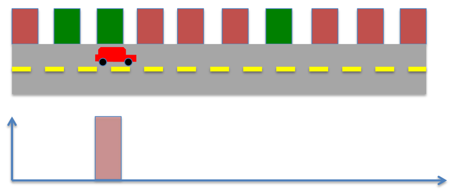
$$ P(C|+) = \frac{P(+|C) P(C)}{P(+|C) P(C) + P(+| NC) P(NC)} , $$

Example 2: Baysean estimation (robot localization)

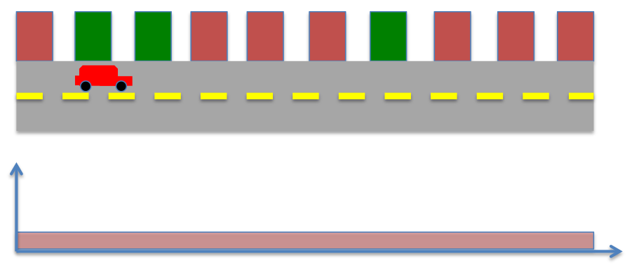
• locations of buildings (red or green) in the world known
• Accurate sensors to detect the color of the building adjacent to the robot
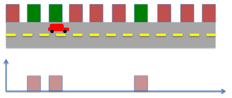
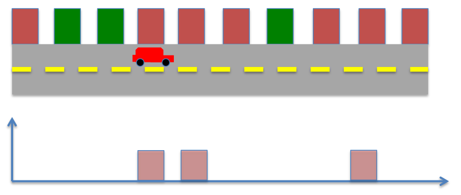
• Locate the robot, given the robot senses green.
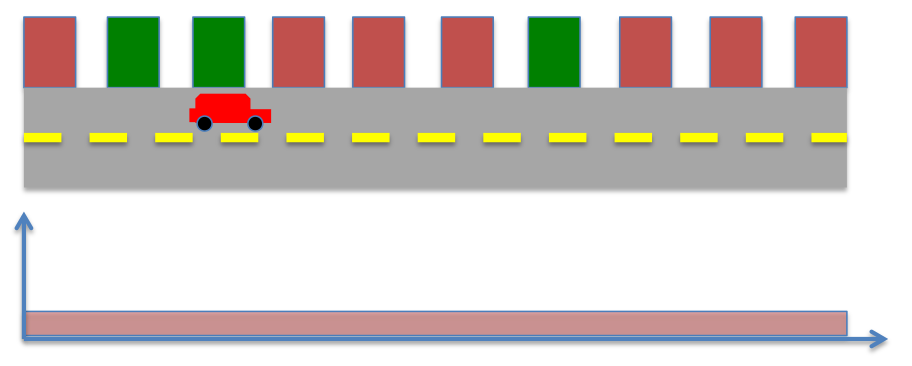
• What is the probability distribution of robot's position after measurement?

$$ P(X)^- = \left[ \begin{array}{cccccccccc} 0.1 & 0.1 & 0.1 & 0.1 & 0.1 & 0.1 & 0.1 & 0.1 & 0.1 & 0.1 \end{array} \right] $$

$$ P(X)^- = \left[ \begin{array}{cccccccccc} 0.1 & 0.1 & 0.1 & 0.1 & 0.1 & 0.1 & 0.1 & 0.1 & 0.1 & 0.1 \end{array} \right] $$$$ P_g(X)= P(g|X)= \left[ \begin{array}{cccccccccc} 0 & 1/3 & 1/3 & 0 & 0 & 0 & 1/3 & 0 & 0 & 0 \end{array} \right] $$$$P(X)^+ = P(X|g) = \frac{P(g|X)P(X)^-}{P(g)} = \frac{P(g|X)P(X)}{\sum_{i=1}^N P(g|X_i)P(X_i) } $$$$ P(X)^+ = P(X|g) = \frac{\left[ \begin{array}{cccccccccc} 0 & 1/3 & 1/3 & 0 & 0 & 0 & 1/3 & 0 & 0 & 0 \end{array} \right] \circ \left[ \begin{array}{cccccccccc} 0.1 & 0.1 & 0.1 & 0.1 & 0.1 & 0.1 & 0.1 & 0.1 & 0.1 & 0.1 \end{array} \right] }{\sum \left( \left[ \begin{array}{cccccccccc} 0 & 1/3 & 1/3 & 0 & 0 & 0 & 1/3 & 0 & 0 & 0 \end{array} \right] \circ \left[ \begin{array}{cccccccccc} 0.1 & 0.1 & 0.1 & 0.1 & 0.1 & 0.1 & 0.1 & 0.1 & 0.1 & 0.1 \end{array} \right] \right)} $$$$ P(X)^+ = P(X|g) = \left[ \begin{array}{cccccccccc} 0 & 1/3 & 1/3 & 0 & 0 & 0 & 1/3 & 0 & 0 & 0 \end{array} \right]$$

Note: The process of multiplying functions and adding them up is also called convolution

• Location certainity after measurement.
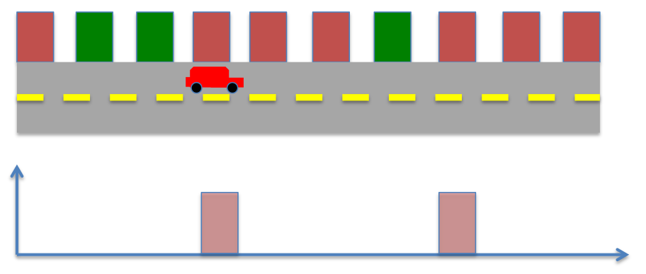
• What is the probability if the robot moves 1 step right?

$$ P(X)^+ = P(X|g) = \left[ \begin{array}{cccccccccc} 0 & 1/3 & 1/3 & 0 & 0 & 0 & 1/3 & 0 & 0 & 0 \end{array} \right]$$

• New prior probability
• Sense again, what is the probability distribution of robot's location now?

$$ P(X)^- = \left[ \begin{array}{cccccccccc} 0 & 0 & 1/3 & 1/3 & 0 & 0 & 0 & 1/3 & 0 & 0 \end{array} \right] $$

$$P(X)^+ = P(X|g) = \frac{P(g|X)P(X)^-}{P(g)} = \frac{P(g|X)P(X)}{\sum_{i=1}^N P(g|X_i)P(X_i) } $$$$ P(X)^+ = \frac{ \left[ \begin{array}{cccccccccc} 0 & 0 & 1/3 & 1/3 & 0 & 0 & 0 & 1/3 & 0 & 0 \end{array} \right] \circ \left[ \begin{array}{cccccccccc} 0 & 1/3 & 1/3 & 0 & 0 & 0 & 1/3 & 0 & 0 & 0\end{array} \right] }{\sum \left( \left[ \begin{array}{cccccccccc} 0 & 0 & 1/3 & 1/3 & 0 & 0 & 0 & 1/3 & 0 & 0 \end{array} \right] \circ \left[ \begin{array}{cccccccccc} 0 & 1/3 & 1/3 & 0 & 0 & 0 & 1/3 & 0 & 0 & 0\end{array} \right] \right)} $$$$ P(X)^+ = \left[ \begin{array}{cccccccccc} 0 & 0 & 1 & 0 & 0 & 0 & 0 & 0 & 0 & 0 \end{array} \right] $$

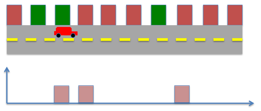
• Probability distribution after 2 step

$$ P(X)^+ = \left[ \begin{array}{cccccccccc} 0 & 0 & 1 & 0 & 0 & 0 & 0 & 0 & 0 & 0 \end{array} \right] $$

Example 2: Baysean estimation (robot localization, scenario 2)

• What is the probability after measurement?

$$ P(X)^- = \left[ \begin{array}{cccccccccc} 0.1 & 0.1 & 0.1 & 0.1 & 0.1 & 0.1 & 0.1 & 0.1 & 0.1 & 0.1 \end{array} \right] . $$

• Bayes' rule

$$P(X)^+ = P(X|g) = \frac{P(g|X)P(X)^-}{P(g)} = \frac{P(g|X)P(X)}{\sum_{i=1}^N P(g|X_i)P(X_i) } $$$$ P(X)^+ = P(X|g) = \left[ \begin{array}{cccccccccc} 0 & 1/3 & 1/3 & 0 & 0 & 0 & 1/3 & 0 & 0 & 0 \end{array} \right]$$

• After movement

$$ P(X)^- = \left[ \begin{array}{cccccccccc} 0 & 0 & 1/3 & 1/3 & 0 & 0 & 0 & 1/3 & 0 & 0 \end{array} \right] $$

• After sensing,

$$P(X)^+ = P(X|r) = \frac{P(r|X)P(X)^-}{P(r)} = \frac{P(r|X)P(X)}{\sum_{i=1}^N P(r|X_i)P(X_i) } $$$$ P_r(X) =P(r|X)= \left[ \begin{array}{cccccccccc} 1/7 & 0 & 0 & 1/7 & 1/7 & 1/7 & 0 & 1/7 & 1/7 & 1/7 \end{array} \right] $$

$$ P(X)^+ = \frac{ \left[ \begin{array}{cccccccccc} 0 & 0 & 0 & 1/21 & 0 & 0 & 0 & 1/21 & 0 & 0 \end{array} \right] }{\sum \left( \left[ \begin{array}{cccccccccc} 0 & 0 & 0 & 1/21 & 0 & 0 & 0 & 1/21 & 0 & 0 \end{array} \right] \right)} = \frac{ \left[ \begin{array}{cccccccccc} 0 & 0 & 0 & 1/21 & 0 & 0 & 0 & 1/21 & 0 & 0 \end{array} \right] }{2/21} $$$$ P(X)^+ = \left[ \begin{array}{cccccccccc} 0 & 0 & 0 & 1/2 & 0 & 0 & 0 & 1/2 & 0 & 0 \end{array} \right] $$

$$ P(X)^+ = \left[ \begin{array}{cccccccccc} 0 & 0 & 0 & 1/2 & 0 & 0 & 0 & 1/2 & 0 & 0 \end{array} \right] $$

Baysian rule for Gaussian distributions

• We could combine movement (dynamics) and measurement information by multiplying their corresponding probabilties.
• If the dependent variable is continuous, we use Gaussian (or normal) distribution.

Gaussian Distributions

• Characterized by a bell-shape curve
• Most physical phenomena follow gaussian-like distributions
• Central limit theorem states that under certain assumptions, mean of random samples drawn from any given distribution converge to a Gaussian/normal distribution when the number of samples become very large.
• Mathematical form of distribution allows us to compute analytical solutions

$$ f(X| \mu, \sigma^2) = \frac{1}{\sqrt{2 \pi \sigma^2}} e^{ - \frac{(X-\mu)^2}{2 \sigma^2}} $$

where, \( \mu \) is the mean and \( \sigma \) is the standard deviation of the distribution.

clc;close all;clear all

X = -10:0.01:10;
mu = 0;
sigma = 1.25;
f_x = 1/sqrt(2*pi*sigma^2) * exp( -(X-mu).^2/(2*sigma^2) );
figure;
plot(X,f_x)
axis([-10 10 0 .4])
xlabel('X')
ylabel('Probability distribution')

Bayesian rule for Gaussian probabilities

Consider two normal probability distributions given by,

$$ f(X| \mu_1, \sigma_1^2) = \frac{1}{\sqrt{2 \pi \sigma_1^2}} e^{ - \frac{(X-\mu_1)^2}{2 \sigma_1^2}} $$

$$ f(X| \mu_2, \sigma_2^2) = \frac{1}{\sqrt{2 \pi \sigma_2^2}} e^{ - \frac{(X-\mu_2)^2}{2 \sigma_2^2}} $$

The Bayesian probability is given by,

$$ f((X| \mu_1, \sigma_1^2)|(X| \mu_2, \sigma_2^2)) = \frac{f(X| \mu_2, \sigma_2^2) f(X| \mu_2, \sigma_2^2)}{\int_{-\infty}^{\infty}f(X| \mu_2, \sigma_2^2) f(X| \mu_2, \sigma_2^2)dX}$$

$$ f((X| \mu_1, \sigma_1^2)|(X| \mu_2, \sigma_2^2)) = \frac{1}{\sqrt{2 \pi \sigma_1^2}} e^{ - \frac{(X-\mu_1)^2}{2 \sigma_1^2}}\frac{1}{\sqrt{2 \pi \sigma_2^2}} e^{ - \frac{(X-\mu_2)^2}{2 \sigma_2^2}} $$

After significant algebra, the final conditional probability, can be represented as,

$$ f(X| \mu_1, \sigma_1^2) | f(X| \mu_2, \sigma_2^2) = f(X| \mu_{12}, \sigma_{12}^2) = \frac{1}{\sqrt{2 \pi \sigma_{12}^2}} e^{ - \frac{(X-\mu_{12})^2}{2 \sigma_{12}^2}} , $$

where,

$$ \sigma_{12}^2 = \frac{\sigma_1^2 \sigma_2^2}{\sigma_1^2+\sigma_2^2} $$

and

$$ \mu_{12} = \frac{\sigma_1^2 \mu_2 + \sigma_2^2 \mu_1}{\sigma_1^2+\sigma_2^2} . $$

Gaussian Example 1: combined probability

• \( \sigma_1 = .8 , \mu_1 = 2 \)
• \( \sigma_2 = .5 , \mu_2 = 4 \)

$$ \sigma_{12}^2 = \frac{\sigma_1^2 \sigma_2^2}{\sigma_1^2+\sigma_2^2}=3.2 $$

and

$$ \mu_{12} = \frac{\sigma_1^2 \mu_2 + \sigma_2^2 \mu_1}{\sigma_1^2+\sigma_2^2}=.66 . $$

clc;close all;clear all
X = -10:0.01:10;
mu1 = .8 ; sigma1 = 2;mu2 = .1 ; sigma2 = 4;
mu12 = (sigma1^2*mu2 + sigma2^2*mu1)/(sigma1^2 + sigma2^2);
sigma12 = sqrt((sigma1^2*sigma2^2)/(sigma1^2 + sigma2^2));
display(['\mu_{12} = ' num2str(mu12) ', \sigma_{12} = ' num2str(sigma12)] )
f1 = 1/sqrt(2*pi*sigma1^2) * exp( -(X-mu1).^2/(2*sigma1^2) );
f2 = 1/sqrt(2*pi*sigma2^2) * exp( -(X-mu2).^2/(2*sigma2^2) );
f12 = 1/sqrt(2*pi*sigma12^2) * exp( -(X-mu12).^2/(2*sigma12^2) );
figure;
plot(X,f12,X,f1,'g--',X,f2,'g--');axis([-10 10 0 .4])
xlabel('X');ylabel('Probability distribution')

\mu_{12} = 0.66, \sigma_{12} = 1.7889

Gaussian Example 2: combined probability

• \( \sigma_1 = -4 , \mu_1 = 2 \)
• \( \sigma_2 = 4 , \mu_2 = 2 \)

$$ \sigma_{12}^2 = \frac{\sigma_1^2 \sigma_2^2}{\sigma_1^2+\sigma_2^2}=2 $$

and

$$ \mu_{12} = \frac{\sigma_1^2 \mu_2 + \sigma_2^2 \mu_1}{\sigma_1^2+\sigma_2^2}=0 . $$

clc;close all;clear all
X = -10:0.01:10;
mu1 = -4 ; sigma1 = 2;mu2 = 4 ; sigma2 = 2;
mu12 = (sigma1^2*mu2 + sigma2^2*mu1)/(sigma1^2 + sigma2^2);
sigma12 = sqrt((sigma1^2*sigma2^2)/(sigma1^2 + sigma2^2));
display(['\mu_{12} = ' num2str(mu12) ', \sigma_{12} = ' num2str(sigma12)] )
f1 = 1/sqrt(2*pi*sigma1^2) * exp( -(X-mu1).^2/(2*sigma1^2) );
f2 = 1/sqrt(2*pi*sigma2^2) * exp( -(X-mu2).^2/(2*sigma2^2) );
f12 = 1/sqrt(2*pi*sigma12^2) * exp( -(X-mu12).^2/(2*sigma12^2) );
figure;
plot(X,f12,X,f1,'g--',X,f2,'g--');axis([-10 10 0 .4])
xlabel('X');ylabel('Probability distribution')

\mu_{12} = 0, \sigma_{12} = 1.4142

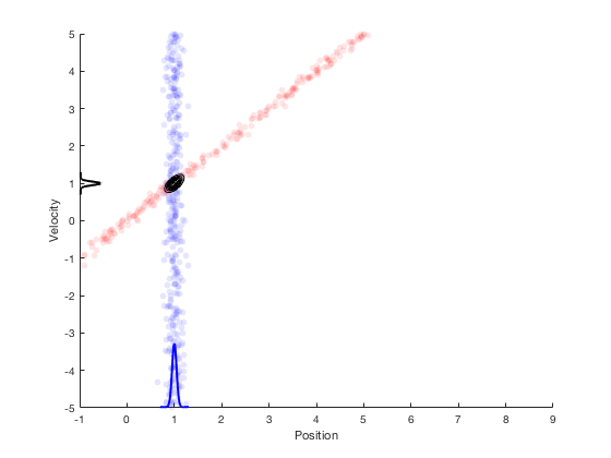
Gaussian 2-D distribution

Multivariate distributions involve multiplication of multiple gaussian distributions,

• Example,

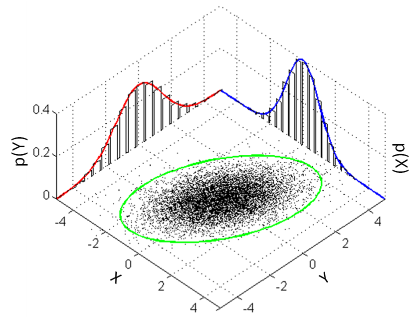
• multivariate distribution in \( k\) dimensions is represented as,

$$ f(X| \mathbf{\mu}, \mathbf{\Sigma}) = \frac{1}{\sqrt{ (2 \pi)^k |\mathbf{\Sigma}| }} e^{ - \frac{1}{2} (X-\mathbf{\mu})^T \mathbf{\Sigma}^{-1} (X-\mathbf{\mu}) }$$

In the special case when \( K = 2 \), we have

$$ \mathbf{\Sigma} = \left[ \begin{array}{cc} \sigma_X^2 & \sigma_{X,Y} \\ \sigma_{X,Y} & \sigma_Y^2 \end{array} \right] $$

where \( \sigma_{X,Y} \) is the second moment between x- and y- variables.

Kalman filter 2-D: Example

• Robot localization, Position measurement only

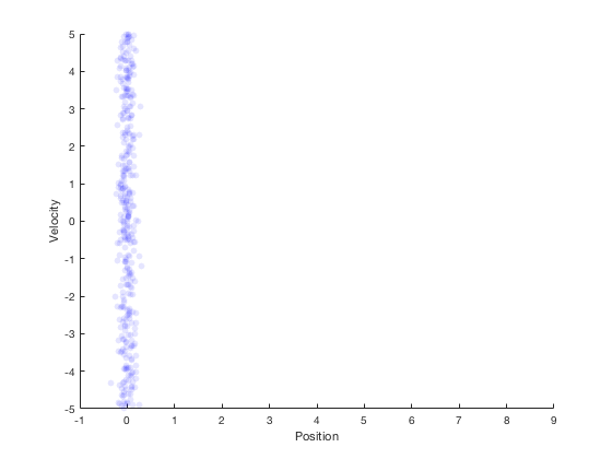
• Robot's next location based on velocity for t = 1 .

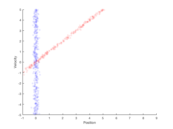
• After movement

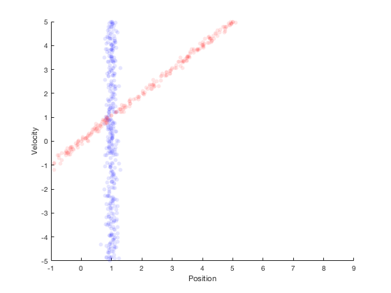
• After multiplying probabilities

Kalman filters: optimality, maximum likelihood

Reframe linear regression problem as follows,

• determining pameters \( \beta_0\) and \( \beta_1 \) such that the likelihood of a given value \( y \) being of the form \( \beta_0 + \beta_1 X \) is maximized. \( e_i = y_i - (\beta_0+ \beta_1 x_i) \). i.e. likelihood of errors coming from a linear fit are

$$ p(e_i| 0, \sigma^2) = \frac{1}{\sqrt{2 \pi \sigma^2}} e^{ - \frac{(y_i - (\beta_0+ \beta_1 x_i))^2}{2 \sigma^2}} $$

$$ p( e_1, e_2, \dots , e_N ) = \underbrace{\Pi}_{i=1~to~n} p(e_i| 0, \sigma^2)$$

$$ p( e_1, e_2, \dots , e_N ) = \underbrace{\Pi}_{i=1~to~n} p(e_i| 0, \sigma^2) = \underbrace{\Pi}_{i=1~to~n} \frac{1}{\sqrt{2 \pi \sigma^2}} e^{ - \frac{(y_i - (\beta_0+ \beta_1 x_i))^2}{2 \sigma^2}} $$$$ \underbrace{Maximize}_{\beta_0,\beta_1}~log(p( e_1, e_2, \dots , e_N )) = \underbrace{Maximize}_{\beta_0,\beta_1}\sum_{i=1}^N \left(- \frac{(y_i - (\beta_0+ \beta_1 x_i))^2}{2 \sigma^2} - \frac{1}{2}log(2 \pi \sigma^2) \right)$$$$ \underbrace{Minimize}_{\beta_0,\beta_1}\sum_{i=1}^N \left(y_i - (\beta_0+ \beta_1 x_i) \right)^2, $$

• Least square solution is the same as maximum likelihood solution if the errors are distributed normally.

Particle filters

• Simulation based filters
• Generate several particles as possible locations of the robot
• Measure states for each particle, and weigh each particle by closeness to true measurement.
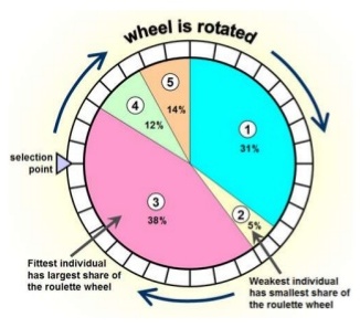
• Resample so particles with larger weight survive

Particle filter for localization