Deriving equations of motion for a 2-R manipulator using MATLAB

Vivek Yadav

Motivation

This document presents Lagrangian techniques to derive equations of motion using symbolic toolbox in MATLAB. Mathematical models are developed to approximate what the actual system may be doing. All mathematical models involve some simplifying assumptions, and typically relaxing these assumptions results in more complex representation of the dynamics of the system. As a result, traditional pen and paper techniques are not sufficient to derive equations representing dynamics of complex systems. Screen shot below presents 2 terms of inertia matrix of 3-D humanoid robot.

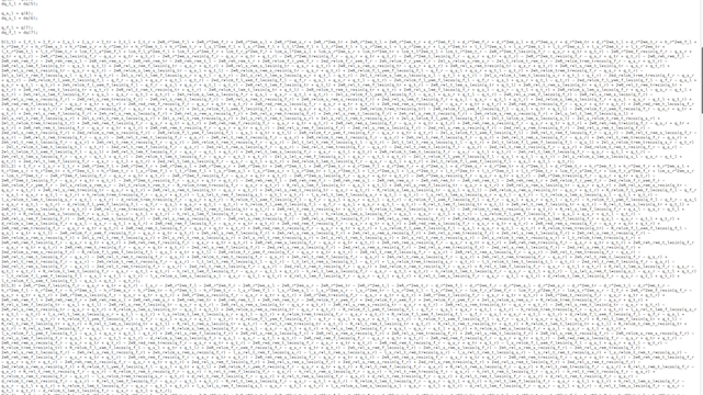
Fig1. - One term in the equation of 3_D humanoid robot.

Thankfully MATLAB, python, and other programming languages offer support for symbolic calculations that can be utilized to automate deriving these equations. In this document, we will derive equations of motion for a 2-link robotic arm (or double pendulum) using MATLAB.

two-link robotic arm model

Consider the model of a simple manipulator shown below. This configuration is also referred to as double pendulum. We assume that the massless links of length $ l_1 $ and $ l_2$ connect masses $ m_1 $ and $m_2$, and the corresponding segment angles are given by $ \theta_1 $ and $ \theta_2 $ . We assume that there is one motor each at each of the joints.

Fig 2. - Simple 2-link manipulator or double pendulum

** We chose angles $ \theta_1 $ and $ \theta_2 $ to describe the system because this represent a representation that requires least number of independent variables to completely describe the system. It is possible to use $ x $ and $ y $ locations of the masses to derive the equations of motion too, however in such cases additional constraints must be imposed on the system to ensure the lengths of links remain constant. Such contraints can be imposed using Pfaffin constraints. However, this method is beyond the scope of this course. For details please refer to chapter 6 in the robotics book by Murray and Sastry. For complex robotic systems or biomechanics simulations, the position vectors are obtained using screw theory or Denavit–Hartenberg parameters. Using appropriate coordinate systems can greatly simplify the equations of motion, however this may not always be possible. For example, human walking model with curved feet cannot be modeled only by ignoring the position and velocity constraint between feet and ground. **

Fig 3. - 7-link biped with curved feet

We will derive the equations of motions using Lagrange method in the following steps,

1. Compute position and velcoties

The first step is to compute position of all the masses in the systems. In this case, we will compute positions of the masses with respect to the origin attached at the base of the manipulator in terms of angles $ \theta_1 $ and $ \theta_2 $.*

$\left[ \begin{array}{c} P_{1,x} \\ P_{1,y} \end{array} \right] = \left[\begin{array}{c} l_1 cos(\theta_1) \\ l_1 sin(\theta_1) \end{array} \right],$

and

$\left[ \begin{array}{c} P_{2,x} \\ P_{2,y} \end{array} \right] = \left[\begin{array}{c} l_1 cos(\theta_1) + l_2 cos(\theta_1 + \theta_2) \\ l_1 sin(\theta_1) + l_2 sin(\theta_1 + \theta_2) \end{array} \right].$

We next compute velocities above using,

$v = \frac{dP}{dt} = \frac{\partial P}{\partial \theta_1} \dot{\theta}_1 + \frac{\partial P}{\partial \theta_2} \dot{\theta}_2 ,$

2. Compute kinetic energy and potential energies of the system.

We next compute potential and kinetic energy of the system. We compute kinetic energy as

$KE = \frac{1}{2} m_1 v_1^T v_1 + \frac{1}{2} m_2 v_2^T v_2$

The potential energy of the system is defined as,

$PE = m_1 g P_{1,y} + m_2 g P_{2,y}$

3. Derive equations of motion

We derive equations of motion by first setting up a Lagrangian $ L $ as

$L = KE - PE$

Equations of motion are then derived using,

$\frac{d}{dt} \left( \frac{\partial L }{\partial \dot{q}} \right) - \frac{\partial L }{\partial q} = \tau,$

where $ q = [ \theta_1, \theta_2]^T $ is the vector of anglular position and velocities, and $ \tau $ is the vector of torques applied by motors at the two joints. After grouping terms appropriately, the equations of motion can be written as

$D (q) \ddot{q} + C(q,\dot{q}) \dot{q} + G(q) = \tau$

$\ddot{q} = D (q)^{-1} (\tau - C(q,\dot{q}) \dot{q} - G(q))$

We can rewrite the equation above as,

$\ddot{q} = \alpha (q,\dot{q}) + \beta (q) \tau ,$

where $ \alpha (q,\dot{q}) = D (q)^{-1} (- C(q,\dot{q}) \dot{q} - G(q)) $ and $ \beta (q) = D (q)^{-1}. $

This form of equation is very common in control of many nonlinear dynamic systems. The special class of systems that have the control input as an linear-additive term to the system dynamics is called control-affine form.

Linearizing equations of motion.

Although almost all systems are non-linear in nature, the system can be approximated by a linear system of equations under certain assumptions. One of the main assumptions is that the system’s postion and velocity are low. This is very common in examples where the task is to stabalize the system against external perturbations. For example, if we want to hold the 2-R manipulator at certain position, say $ q_0 $, then we may assume that the result of external perturbation is small. Therefore, we can apply taylor series expansion on the terms of the matrix about the stable point $ q_0 $. First as the system is at equilibirum at $ q_0 $ , $ \dot{q} = 0 , \ddot{q} = 0 $. Therefore,

$0 = \alpha (q_0,0) + \beta (q_0) \tau_0 ,$

$\tau_0 = - \beta (q_0) ^{-1}\alpha (q_0,0) .$

Recall Taylor series expansion for a function of two variables,

$f(x+\delta x,y+\delta y) \approx f(x ,y) + \left. \frac{\partial f}{ \partial x} \right|_{(x,y)} \delta x + \left. \frac{\partial f}{ \partial y} \right|_{(x,y)} \delta y .$

Using the equation above, about $ q = q_0 $ and $ \dot{q} = 0 $,

$\delta \ddot{q} = \alpha (q_0,0) + \left. \frac{\partial \alpha}{ \partial q} \right|_{(q_0,0)} \delta q + \left. \frac{\partial \alpha}{ \partial q} \right|_{(q_0,0)} \delta \dot{q} + \left( \beta (q_0,0) + \left. \frac{\partial \beta}{ \partial q} \right|_{(q_0,0)} \delta q \right) \left( \tau_0 + \delta \tau_0 \right) + H.O.T,$

Rearranging and ignoring the higher order terms,

$\delta \ddot{q} = \underbrace{\left. \frac{\partial \alpha}{ \partial q} \right|_{(q_0,0)} \delta q + \left. \frac{\partial \alpha}{ \partial q} \right|_{(q_0,0)} \delta \dot{q} + \left. \frac{\partial \beta}{ \partial q} \right|_{(q_0,0)} \delta q \tau_0 }_{\text{Linear in } \delta q \text{ and } \delta \dot{q}} + \underbrace{ \beta (q_0) \delta \tau_0 }_{\text{Linear in } \delta \tau_0},$

Therefore, the equations of motion can be expressed as a simpler linear dynamic system about $ q_0 $ and $ \dot{q} = 0 $.

In cases where the system in not control affine, the Taylor series expansion can be used as follows,

$\ddot q_0 + \delta \ddot q = f(q_0+\delta q,u_0+\delta u) \approx f(q_0 ,u_0) + \left. \frac{\partial f}{ \partial q} \right|_{(q_0,u_0)} \delta q + \left. \frac{\partial f}{ \partial u} \right|_{(q_0,u_0)} \delta u .$

Noting that $ \ddot q_0 = f(q_0 ,u_0) $,

$\delta \ddot q = \left. \frac{\partial f}{ \partial q} \right|_{(q_0,u_0)} \delta q + \left. \frac{\partial f}{ \partial u} \right|_{(q_0,u_0)} \delta u .$

Note: Partial derivatives are computed using matrix derivatives as shown here.

MATLAB implementation of the code.

We almost never perform these calculations by hand. Instead, we use MATLAB’s symbolic toolbox to implement reusable functions to perform the calculations above. The code and accompanying functions can be downloaded from the github repository for MATLAB codes or google drive.

clc
close all
clear all

addpath Screws
addpath fcn_support
% Defining symbols
syms m1 m2 l1 l2 q1 q2 dq1 dq2 ddq1 ddq2 tau1 tau2 g real
syms q10  q20

% Position vectors



P1 = [  l1 * cos(q1);
    l1 * sin(q1)];

P2 = [  l1 * cos(q1) + l2 * cos(q1+q2);
    l1 * sin(q1)+ l2 * sin(q1+q2)];

q_v = [q1;q2];
dq_v = [dq1;dq2];
% 

% Taking derivative to compute velocities
V1 = get_vel(P1 ,q_v,dq_v);
V2 =get_vel(P2,q_v,dq_v);

% Computing Kinetic energy and potential energy
KE1 =simplify(1/2*m1*V1'*V1);
KE2 =simplify(1/2*m2*V2'*V2);

PE1 = m1*g*P1(2);
PE2 = m2*g*P2(2);

% Define Lagrangian
KE_total = KE1 + KE2;
PE_total = PE1 + PE2;


[D,C,G] = get_mat(KE_total, PE_total, q_v,dq_v);
D = simplify(D);
C = simplify(C);
G = simplify(G);


% Now express this in the form of dx/dt = f(x,u)
x = [q1;q2;dq1;dq2]; % Vector of state space
ddq0 = [0;0]; % Vector of SS joint accelerations
x0 = [q10;q20;0;0]; % Vector of SS joint angles and velocites
tau_v = [tau1;tau2]; % Vector of torques
% Function to calculate Linearized representation
[A_lin,B_lin] = linearize_DCG(D,C,G,x,tau_v,x0,ddq0);
A_lin = simplify(A_lin)
B_lin = simplify(B_lin)