Control synthesis

Vivek Yadav

1. Recap

We previously studied how to represent system dynamics in a state-space form.

$\frac{d x(t) }{dt} = A x(t) + B u(t) .$ $y = C x + D u$

We saw that for continuous systems, the states of the system converge to 0 if the real parts of all the eigen values of $ A$ are negative, and for discrete system the states converge to 0 if the real parts of the eigen values of $ A$ are less than 1. We also saw how these two conditions are equivalent by discretizing a continuous system. Next we reviewed how to simulate dynamic systems and simulated dynamic systems to study their behavior. We next derived conditions for a linear time-invariant system to be controllable. With these tools, we can now proceed to design control systems for most applications. A typical control systems design process looks as follows,

Identify the states, control and measurement variables.
Use physics to derive equations of motion (or system dynamics) relating the evolution of states with control signals.
Derive equations to reconstruct states from measurements.
Test if the system is controllable and observable.
Design observer and choose appropriate control scheme and test if the chosen control scheme achieves the desired behavior.

2. Controller synthesis

A controls engineer’s task is to design the observer or estimator and to choose the appropriate control scheme. Most control schemes are divided into two broad categories feedback and feedforward control. Feedback control refers to a control scheme that takes in the current states of the system, compares it to desired behavior and applies a corrective input to the system. Feedforward control refers to a control scheme where the controller applies a precomputed sequence of control to the system. Although these definitions are accurate, they are not sufficient to characterize different behaviors of a control system. We will divide the controller tasks into 4 broad categories,

Regularization (feedback): Regularization refers to driving states of the system to 0, or to a fixed desired value. The later is achieved by formulating an error dynamic relation where the states of the system are the error between the actual and desired states of the system. Designing optimal regulator involves parametrizing the control law and applying first variance principles to compute the desired control scheme.
Stabilization (feedback): Stabilization refers to the process of cancelling the effects of any disturbance or errors so the states of the system remain at a desired stable point. Although, colloquially stabilization refers to stabilizing about a fixed point (rate of change of position = 0), stabilizing control can also cancel the effects of perturbations about a desired trajectory. We will use the second definition of stalizing control for control systhesis/design purpose.
Tracking: Tracking control refers to the controller is tasked to make the states of the system track a desired state trajectory or path. Tracking control can be implemented as a feedforward control where one computes the sequence of control inputs based on the desired states and applies the control to the system. However, this typically results in erroneous performance. A tracking control is typically implemented along with a stabilizing control which cancels out the effect of any processes that may act to deviate the controller from its desired state trajectory.
Trajectory computing or path planning: The controller objective is to achieve a certain behavior of a system. This behavior can be as simple as driving the states of the system to 0, to as complex as achieve periodic behavior of the states of the system. Typically, regularization and stabilization task the controller to achieve a desired asymptotic performance, they do not dictate how the asymptotic performance is achieved. Trajectory planning refers to the the task of planning the trajectory from an initial to a desired state value under external constraints. Early approaches to trajectory planning involved obtaining first variance conditions to obtain a set of equations the optimal control scheme should satisfy and solving them. However, solving these equations is not always easy. An alternate method is to use numerical techniques to compute an approximate trajectory or path, and then use a stabilizing control around this trajectory. Typically, this process involves approximating the control input by polynomials and converting the control objective into a nonlinear programming task. The trajectory thus generated need not be one that could be followed accurately by the controller while satisfying system dynamics.

The above classification of controllers is not the only classification, but is one that is based on the task of the controller. Researchers have further developed and hence classified these controllers based on how the controllers achieve their goal. A few examples are, sliding mode control, output-feedback control, optimal-feedback control, sliding mode control, linear quadratic control, pole placement, etc. We will study these schemes later in the course, but for now, we will work with perhaps the simplest; pole-placement control scheme. Pole-placement refers to the control scheme that achieves its objective by modifying the eigen values (and hence poles) of the system. Recall, poles of the system are solutions of the characteristic equation of the system matrix, the roots of the denomenator in the transfer function and the eigen values of the system dynamics matrix.

We will first design controller when full-state feedback refers to control design when all the states of the system are available to the controller for design.

** Note: A control systems designer should always check if the system he/she is designing control for is controllable with the given set of actuators, and if the measurements provide information needed to design the controller. **

We will first work with the case when full-state feedback is available.

3. Full-state feedback of discrete system

Consider the dynamic system given by,

$x[k+1] = Ax[k] +B u[k]$

under the assumption that all states are available for controller design. Say we choose control $ u[k] = - K x[k] $, where $ K $ is a matrix of gains of appropriate size. The system dynamics equation changes as,

$x[k+1] = Ax[k] +B (- K x[k]) .$

Rearranging terms gives,

$x[k+1] = (A - BK) x[k] .$

Recall, solution of $ x[k+1] = (A - BK) x[k] $ is

$x[k] = (A-BK)^k x_o .$

Therefore, if the real part of all the eigen values of $ (A-BK) $ are less than 1, the states $ x $ of the system go to 0.

Proof: As before, we will apply Lyapunov method to verify that the controller $ u[k] = -Kx[k] $ always drives the states of the system to 0. In Lyapunov method, first a positive function is defined, and difference methods are used to verify if the applied control drives the system to 0. Any control scheme that decreases the Lyapunov function for all values of $ x [k] $ except $ x [k] = 0 $ results in a system that drives the value of the states to 0.

Consider the error function,

$L(x[k]) = \frac{1}{2} x[k]' x[k]$

As $ L(x) $ is always positive, it satisifies the criteria that the Lyapunov function is positive. We will next investigate if the Lyapunov is decreasing. As the system dynamics is discrete, the Lyapunov function is discrete too. Therefore, instead of taking the derivative, we compute a difference of Lyapunov,

$\Delta L = L(x[k+1]) - L(x[k]) = \frac{1}{2} ( x[k+1]' x[k+1] - x[k]' x[k] )$

Substituting $ x[k+1] = Ax[k] +B u[k] $ gives,

$\Delta L = \frac{1}{2} ( (Ax[k] +B u[k])' (Ax[k] +B u[k]) - x[k]' x[k] )$ $\Delta L = \frac{1}{2} [ ((A-BK)x[k])' ((A-BK)x[k]) - x[k]' x[k] ]$ $\Delta L = \frac{1}{2} x[k]' [ (A-BK)' (A-BK) - I ] x[k]$

If all the eigen values of $ [ (A-BK)’ (A-BK) - I ] $ have negative real parts, i.e. $ (A-BK) $ has all eigen values whose real parts’ absolute value are less than 1. Therefore, if $ (A-BK) $’s eigen values’ real parts are all less than 1, then the states of the system go to 0. Further, the Lyapunov function is decreasing for all values of the states except when $ x[k] = 0 $.

4. Full-state feedback of continuous system

Consider the dynamic system given by,

$\dot{x} = Ax +B u$

under the assumption that all states are available for controller design. Say we choose control $ u = - K x $, where $ K $ is a matrix of gains of appropriate size. The system dynamics equation changes as,

$\dot{x} = Ax +B (- K x) .$

Rearranging terms gives,

$\dot{x} = (A - BK) x .$

Recall, solution of $ \dot{ x} = (A - BK) x $ is

$x(t) = e^{(A-BK)t}x_o .$

Therefore, if the real part of all the eigen values of $ (A-BK) $ are negative, then the states $ x $ of the system go to 0.

Proof:

We previously showed using linear algebra that if the real part of all the eigen values of $ (A-BK) $ are negative, then the states $ x $ of the system go to 0. We will now apply another technique, Lyapunov method to prove the same. In Lyapunov method, a control designer first defines a function that is always positive, and then applies a control that always decreases this function for all values except the desired value. The function that the user defines is typically squared deviation from desired states, and in some cases may have a physical interperetation as energy of the system. Therefore, a controller that always decreases a positive function except when the states are the desired value, will drive it to the desired value.

Consider the error function,

$L(x) = \frac{1}{2} x' x$

As $ L(x) $ is always positive, it satisifies the criteria that the Lyapunov function is positive. We will next investigate if the Lyapunov is decreasing by taking its derivative with respect to time,

$\frac{dL(x)}{dt} = \frac{1}{2} ( \dot{x}' x + x' \dot{x} ) = x' \dot{x}.$

As $ \dot{x} = Ax +B u $, we get

$\frac{dL(x)}{dt} = x' (Ax + Bu).$

Noting that $ u = - Kx $,

$\frac{dL(x)}{dt} = x' (Ax + B(-Kx)) = x' (A-BK) x.$

If all the eigen values of $ (A-BK) $ have negative real parts then $x’ (A-BK) x $ is decreasing for all values of $ x $ except when $ x = 0 $, which is our desired value. Therefore, as long as $ x \neq 0 $, the states of the system go towards 0.

** Note: Lyapunov methods are not typically applied for linear systems because the conditions for the states to go to zero for continuous and discrete system can be derived from linear algebra. Lyapunov methods are more useful when studying nonlinear systems. **

5. Pole placement:

Choosing $ K $ such that the eigen values of $ A - B K $ have negative real parts results in a system whose states go to zero. However, it is not yet clear how to choose the $ K $ such that $ A - B K $ has eigen values as the user desires. Ackermann’s Formula gives one method of doing pole placement in one step. The controller gain $ K $ is given by,

$K = \left[ \begin{array}{cccc}0 & \dots & 0 & 1 \end{array} \right]_{1 \times n} M_A^{-1} \Phi(A)$

where $ M_A = \left[ \begin{array}{ccccc} B & AB & A^2B & \dots & A^{n-1}B \end{array} \right] $ is the controllability matrix, $ \Phi(A) $ is the characteristic polynomial of the closed loop poles evaluated for the matrix $ A $.

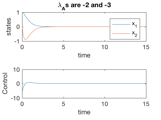
Pole placement: Regulator example

Consider the double integrator system $ \ddot{x} = u $. This system can be written in state space form as,

$\frac{d}{dt}\left[ \begin{array}{c} x_1 \\ x_2 \end{array} \right] = \left[ \begin{array}{cc} 0 & 1 \\ 0 & 0 \end{array} \right]\left[ \begin{array}{c} x_1 \\ x_2 \end{array} \right] + \left[ \begin{array}{c} 0 \\ 1 \end{array} \right] u$

Say, we want to choose the gain $ K $ for the control $ u $ such that the poles of the system are at $-2$ and $-3$. The controllability matrix $ M_A $ is given by

$M_A = \left[ \begin{array}{cc} B & AB \end{array} \right] = \left[ \begin{array}{cc} \left[ \begin{array}{c} 0 \\ 1 \end{array} \right] & \left[ \begin{array}{cc} 0 & 1 \\ 0 & 0 \end{array} \right]\left[ \begin{array}{c} 0 \\ 1 \end{array} \right] \end{array} \right]$ $M_A = \left[ \begin{array}{cc} 0 & 1 \\ 1 & 0 \end{array} \right] .$

The characteristic polynomial is given by,

$\Phi(\lambda) = (\lambda - \lambda_1) (\lambda - \lambda_2) = (\lambda - (-2)) (\lambda - (-3)) = \lambda^2 + 5 \lambda + 6 .$

Therefore, $\Phi(A) = A^2 + 5 A + 6 = \left[ \begin{array}{cc} 0 & 1 \\ 0 & 0 \end{array} \right]^2 + 5\left[ \begin{array}{cc} 0 & 1 \\ 0 & 0 \end{array} \right] + 6 \left[ \begin{array}{cc} 1 & 0 \\ 0 & 1 \end{array} \right] = \left[ \begin{array}{cc} 6 & 5 \\ 0 & 6 \end{array} \right]$

$K = \left[ \begin{array}{cccc}0 & \dots & 0 & 1 \end{array} \right]_{1 \times n} M_A^{-1} \Phi(A)$ $K = \left[ \begin{array}{cc}0 & 1 \end{array} \right] \left[ \begin{array}{cc} 0 & 1 \\ 1 & 0 \end{array} \right]^{-1} \left[ \begin{array}{cc} 6 & 5 \\ 0 & 6 \end{array} \right] = \left[ \begin{array}{cc}6 & 5 \end{array} \right]$

The same technique can be applied using MATLAB’s built in function, ‘place’ or ‘acker’. Recall controlability matrix can be obtained using ctrb(A,B) and polynomial functions can be evaluated using polyvalm(coeffs,A)

The code below implements the controller scheme presented above.

clc
close all
clear all


A = [0 1; 0 0];
B = [0  ;1];

M_A = ctrb(A,B);
phi_A = polyvalm([1 5 6],A);
K = [0 1]*inv(M_A)*phi_A;

[v,d] = eig(A-B*K);


control = @(x)[-K*([x(1,:);x(2,:)])];
sys_dyn = @(t,x)[A*x + B*control(x)];
Tspan = 0:0.1:15;
x0 = [1;0];

[t,x] = ode45(sys_dyn,Tspan,x0);

figure;
subplot(2,1,1)
plot(t,x)
legend('x_1','x_2')
ylabel('states')
xlabel('time')
title(['\lambda_As are ' num2str(d(1,1)) ' and ' num2str(d(2,2))])
subplot(2,1,2)
plot(t,control(x'))
ylabel('Control')
xlabel('time')

Fig 1. - Pole-placement controller for simple regulator

Pole placement: Set point tracking and steady state error

We will now investigate the performance pole-placement technique for tasks that require the states to go to a non-zero value. This is also referred to as set-point control. We assume that we want to drive the states of the system $ \dot{x} = Ax +B u $ to $ x_{des} . $ We define an error between the current and desired states $ e $ as

$e = x - x_{des}.$

The states $ x $ can be rewritten as $ e = x - x_{des}. $ The system dynamics now become,

$\dot{e} + \dot{x}_{des} = A(e + x_{des}) +B u$

Choosing $ u = - K (x - x_{des}) = - Ke $ gives,

$\dot{e} + \dot{x}_{des} = A(e + x_{des}) +B (- Ke) = (A-BK)e + Ax_{des}$

At steady state, $ \dot{e} = 0 $ and $ \dot{x}_{des} = 0 $, therefore,

$0 = (A-BK)e_{ss} + Ax_{des}$ $e_{ss} = - (A-BK)^{-1}Ax_{des}$

Therefore, the steady state error is not 0, futher driving the error to 0 will require a very large values for controller gains $ K $.

One way to fix this issue is to append the system by adding an additional state, the integral of error. Therefore, at steady state, for this system, the error between the actual and desired state goes to zero.

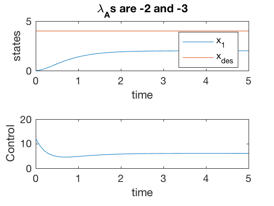
Pole placement: Steady state error example.

** Spring-mass-damper ** Consider a spring-mass-damper second order system given by

$\ddot{x} + 2 \dot{x} + 3 x = u.$

The system can be written in state space form as

$\frac{d}{dt}\left[ \begin{array}{c} x_1 \\ x_2 \end{array} \right] = \left[ \begin{array}{cc} 0 & 1 \\ -3 & -2 \end{array} \right]\left[ \begin{array}{c} x_1 \\ x_2 \end{array} \right] + \left[ \begin{array}{c} 0 \\ 1 \end{array} \right] u$

Say we want to place the poles of the system at -2 and -3, which gives a $ K = \left[ \begin{array}{cc} 3 & 3 \end{array} \right] $. From calculations above, it can be shown that the steady state error is half the desired value. This is also confirmed by the simulations below.

clc
close all
clear all


A = [0 1; -3 -2];
B = [0  ;1];

M_A = ctrb(A,B);
phi_A = polyvalm([1 5 6],A);
K = [0 1]*inv(M_A)*phi_A;

[v,d] = eig(A-B*K);


control = @(x)[-K*([x(1,:)-4;x(2,:)])];
sys_dyn = @(t,x)[A*x + B*control(x)];
Tspan = 0:0.1:5;
x0 = [0;0];

[t,x] = ode45(sys_dyn,Tspan,x0);

figure;
subplot(2,1,1)
plot(t,x(:,1),t,4*ones(size(t)))
legend('x_1','x_{des}')
ylabel('states')
xlabel('time')
axis([0 5 0 5])
title(['\lambda_As are ' num2str(d(1,1)) ' and ' num2str(d(2,2))])
subplot(2,1,2)
plot(t,control(x'))
ylabel('Control')
xlabel('time')

Fig 2. - Pole-placement controller's performance for obtaining a fixed set-point

Pole placement: Steady state error with Integrator.

To improve the performance for set-point control, we introduce an additional state into the system, the integral of error between current position and desired set point.

$e_I = \int_0^t (x - x_{des})dt.$

By adding this additional state, the system changes as,

$\frac{d}{dt} \left[ \begin{array}{c} e_I \\ x \end{array} \right] = \left[ \begin{array}{cc} 0 & 1 \\ 0 & A \end{array} \right] \left[ \begin{array}{c} e_I \\ x \end{array} \right] + \left[ \begin{array}{c} 0 \\ B \end{array} \right] U - \left[ \begin{array}{c} x_{des} \\ 0 \end{array} \right]$

Note, in this case at steady state, the derivatives of the states are zero, therefore, the state $ x \rightarrow x_{des}.$ The control in this case is given by

$u = -K \left( \left[ \begin{array}{c} e_I \\ x \end{array} \right] - \left[ \begin{array}{c} 0 \\ x_{des} \end{array} \right] \right).$

** Note: While adding additional one should be careful to not introduce redundant state information. For example, in a double integrator system, the information about the state is already included, therefore, adding integral of velocity as an additional state will introduce redundancy in the system. Therefore, we add integral of state deviation from the desired value alone as the additional state. **

** Spring-mass-damper with error integrator **

The spring mass damper presented above, with integrator as an additional state can be represented as,

$\frac{d}{dt} \left[ \begin{array}{c} e_I \\ x_1 \\ x_2 \end{array} \right] = \left[ \begin{array}{ccc} 0 & 1 & 0\\ 0 & 0 & 1\\ 0 & -3 & -2 \end{array} \right] \left[ \begin{array}{c} e_I \\ x_1 \\ x_2 \end{array} \right] + \left[ \begin{array}{c} 0 \\0 \\ 1 \end{array} \right] U + \left[ \begin{array}{c} -x_{des} \\ 0 \\ 0 \end{array} \right],$

with control $ u $ given by,

$u = -K \left( \left[ \begin{array}{c} e_I \\ x_1 \\ x_2 \end{array} \right] - \left[ \begin{array}{c} 0 \\ x_{des} \\ 0 \end{array} \right] \right).$

clc
close all
clear all


A = [0 1 0; 0 0 1;0 -3 -2];
B = [0 ; 0 ;1];

p = [-2;-3;-4];
K = place(A,B,p);

[v,d] = eig(A-B*K);

x_des = 4;
control = @(x)[-K*([x(1,:);x(2,:)-x_des; x(3,:)])];
sys_dyn = @(t,x)[A*x + B*control(x)-[x_des;0;0]];
Tspan = 0:0.1:5;
x0 = [0;0;0];

[t,x] = ode45(sys_dyn,Tspan,x0);

figure;
subplot(2,1,1)
plot(t,x(:,2),t,x_des*ones(size(t)))
legend('x_1','x_{des}')
ylabel('states')
xlabel('time')
title(['\lambda_As are ' num2str(d(1,1)) ', ' num2str(d(2,2)) ' and ' num2str(d(3,3))])
subplot(2,1,2)
plot(t,control(x'))
ylabel('Control')
xlabel('time')

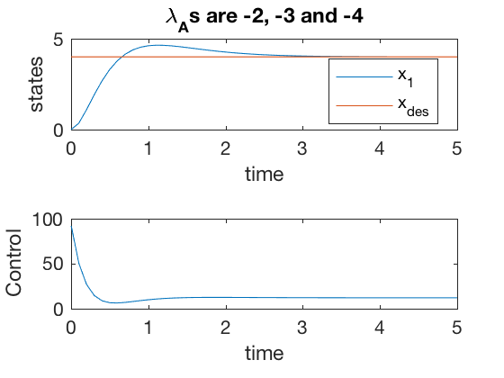
Fig 3. - Pole-placement controller's performance improves with addition of integrator state term.

From simulations above, it can be seen that the error between the desired and actual states go to zero, and performance is much better than the case when the integrator was not used as an additional state. However, note that the amplitude of the required control signal is very high at start $ 100 $, and this control has to be achieved at the start.

Tracking

We will next investigate the performance of the pole-placement technique for tracking a time-dependent signal. Consider the system from before $ \dot{x} = Ax + Bu $, and say we apply the control law based on difference between the actual and desired state values $ u = -K ( x - x_{des}) $. As before, consider the spring mass system given by,

$\ddot{x} + 2 \dot{x} + 3 x = u.$

The system can be written in state space form as

Say we want to track a time varying signal, $ x_{des} = sin( \omega t ) $. The control in this case can be written as,

$u = \left( \left[ \begin{array}{c} x_1 \\ x_2 \end{array} \right] - \left[ \begin{array}{c} sin(\omega t) \\ \omega cos(\omega t) \end{array} \right] \right)$

clc
close all
clear all

A = [0 1; -3 -2];
B = [0  ;1];

p = [-2;-3];
K = place(A,B,p);
[v,d] = eig(A-B*K);

w = 2;

control = @(t,x)[-K*(x - [sin(w*t);w*cos(w*t)] )];
sys_dyn = @(t,x)[A*x + B*control(t,x)];
Tspan = 0:0.1:25;
x0 = [0;0];

[t,x] = ode45(sys_dyn,Tspan,x0);
figure;
subplot(2,1,1)
plot(t,x(:,1),t,sin(w*t))
legend('x_1','sin(t)')
title(['\lambda_A are ' num2str(d(1,1)) ' and ' num2str(d(2,2))])
subplot(2,1,2)
plot(t',control(t',x'))
axis([0 25 -10 10])

err1 = x(:,1)-sin(w*t);

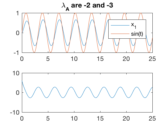
Fig 4. - Pole-placement controller's performance for tracking a time-varying signal.

Simulation results indicate that the error between the desired and actual state values is high, and the tracking performance is poor. The required control for this process is also high, and as before starts off at a non-zero value. For set point tracking, we were able to append the states with integral of error, and improve performance. Lets investigate if the same trick helps improve performance for tracking time-varying signals.

** Spring-mass-damper with error integrator **

The spring mass damper presented above, with integrator as an additional state can be represented as,

with control $ u $ given by,

$u = -K \left( \left[ \begin{array}{c} e_I \\ x_1 \\ x_2 \end{array} \right] - \left[ \begin{array}{c} 0 \\ x_{des} \\ \dot{x}_{des} \end{array} \right] \right).$

A = [0 1 0; 0 0 1;0 -3 -2];
B = [0 ;0 ;1];

p = [-2;-3;-4];
K = place(A,B,p);
[v,d] = eig(A-B*K);

w = 2;

control = @(t,x)[-K*(x - [zeros(size(t));sin(w*t);w*cos(w*t)] )];
sys_dyn = @(t,x)[A*x + B*control(t,x)-[sin(w*t);0;0] ];
Tspan = 0:0.1:25;
x0 = [0;0;0];

[t,x] = ode45(sys_dyn,Tspan,x0);
figure;
subplot(2,1,1)
plot(t,x(:,2),t,sin(w*t))
axis([0 25 -1 1])
legend('x_1','sin(t)')
title(['\lambda_As are ' num2str(d(1,1)) ', ' num2str(d(2,2)) ' and ' num2str(d(3,3))])
subplot(2,1,2)
plot(t',control(t',x'))
err2 = x(:,2)-sin(w*t);
axis([0 25 -10 10])

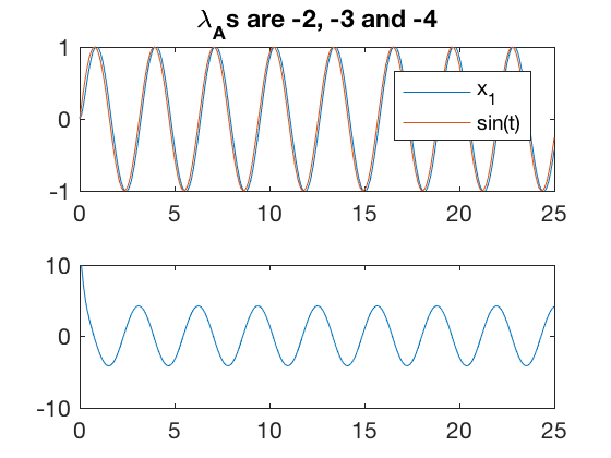
Fig 4. - Pole-placement controller's performance for tracking a time-varying signal improves by adding an integrator term to state space.

From simulations above, the tracking performance has significantly improved. However, the control still starts at a non-zero value. Most controllers cannot apply a non-zero control value when they start from idle conditions, further, most controllers have limits on how large control signal they can apply.

Actuator considerations:

Actuators are physical devices that apply the commanded control input to the plant. Most actuators have certain limitations, and it is crucial to design control systems with special consideration to actuators. We will consider 2 particular aspects of actuators,

Actuator constraints: Actuator contraints refer to the maximum and minimum values that could be achieved by an actuator. In most cases, if the required control to achieve desired performance is beyond these bounds, then the desired behavior cannot be achieved. Therefore, it is important to know what the system is being designed for, and to make sure the actuators can apply the required control commands.
Actuator dynamics: Actuator dynamics refers to the characteristic that most actuators do not have an infinite bandwidth, i.e. they have a response delay and cannot apply a large control signal starting from rest. In such cases, it is possible to append control to the state-space as a first order system, with commanded control being the new control input.

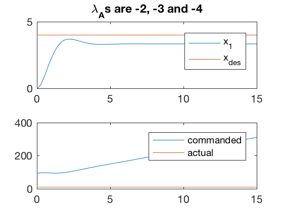
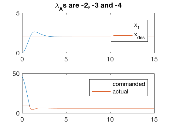
1. Actuator contraints

As mentioned, if the actuator cannot apply the commanded control, the desired behavior may not be reachable. Examples below illustrate 2 cases where the controller is unable to apply the commanded input. In one case, the controller is able to reduce the error by performing at the saturation for some time. However, such behaviors are not desirable, and can usually result in overheating or other issues which can damage the controller. Therefore, it is important to choose the actuators before desining the complete control system. A poor choice can limit the capabilities of the overall system.

A = [0 1 0; 0 0 1;0 -3 -2];
B = [0 ;0 ;1];

p = [-3;-4;-2];
K = place(A,B,p);
[v,d] = eig(A-B*K);

x_des= 4;

control_saturate = @(x)[sign(x).*min(abs(x),10)];
control = @(t,x)[-K*(x - [zeros(size(t));x_des*ones(size(t));zeros(size(t)) ])];
sys_dyn = @(t,x)[A*x + B*control_saturate(control(t,x))-[x_des;0;0] ];
Tspan = 0:0.1:15;
x0 = [0;0;0];

[t,x] = ode45(sys_dyn,Tspan,x0);
figure;
subplot(2,1,1)
plot(t,x(:,2),t,x_des*ones(size(t)))
axis([0 15 0 5])
legend('x_1','x_{des}')
title(['\lambda_As are ' num2str(d(1,1)) ', ' num2str(d(2,2)) ' and ' num2str(d(3,3))])
subplot(2,1,2)
plot(t',control(t',x'),t',control_saturate(control(t',x')))
legend('commanded','actual')
%axis([0 25 -10 10])

Fig 5. - Pole-placement controller performs well under saturation if error between commanded and maximum value is not large.

A = [0 1 0; 0 0 1;0 -3 -2];
B = [0 ;0 ;1];

p = [-3;-4;-2];
K = place(A,B,p);
[v,d] = eig(A-B*K);

x_des= 2;

control_saturate = @(x)[sign(x).*min(abs(x),10)];
control = @(t,x)[-K*(x - [zeros(size(t));x_des*ones(size(t));zeros(size(t)) ])];
sys_dyn = @(t,x)[A*x + B*control_saturate(control(t,x))-[x_des;0;0] ];
Tspan = 0:0.1:15;
x0 = [0;0;0];

[t,x] = ode45(sys_dyn,Tspan,x0);
figure;
subplot(2,1,1)
plot(t,x(:,2),t,x_des*ones(size(t)))
axis([0 15 0 5])
legend('x_1','x_{des}')
title(['\lambda_As are ' num2str(d(1,1)) ', ' num2str(d(2,2)) ' and ' num2str(d(3,3))])
subplot(2,1,2)
plot(t',control(t',x'),t',control_saturate(control(t',x')))
legend('commanded','actual')
%axis([0 25 -10 10])

Fig 6. - Pole-placement controller performs poorly under saturation if error between commanded and maximum value is large.

A = [0 1 0; 0 0 1;0 -3 -2];
B = [0 ;0 ;1];

p = [-2;-3;-4];
K = place(A,B,p);
[v,d] = eig(A-B*K);

w = 2;

control_saturate = @(x)[sign(x).*min(abs(x),5)];
control = @(t,x)[-K*(x - [zeros(size(t));sin(w*t);w*cos(w*t)] )];
sys_dyn = @(t,x)[A*x + B*control_saturate(control(t,x))-[sin(w*t);0;0] ];
Tspan = 0:0.1:25;
x0 = [0;0;0];

[t,x] = ode45(sys_dyn,Tspan,x0);
figure;
subplot(2,1,1)
plot(t,x(:,2),t,sin(w*t))
axis([0 25 -1 1])
legend('x_1','sin(t)')
title(['\lambda_As are ' num2str(d(1,1)) ', ' num2str(d(2,2)) ' and ' num2str(d(3,3))])
subplot(2,1,2)
plot(t',control(t',x'),t',control_saturate(control(t',x')))
legend('commanded','actual')
err2 = x(:,2)-sin(w*t);
axis([0 25 -10 10])

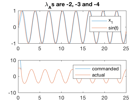
Fig 7. - Pole-placement controller performs well for tracking under saturation if error between commanded and maximum value is not large.

2. Actuator dynamics

Actuator dynamics refers to the characteristic that most actuators do not have an infinite bandwidth, i.e. they have a response delay and cannot apply a large control signal starting from rest. In such cases, it is possible to append control to the state-space as a first order system, with commanded control being the new control input. Say the actuator dynamics are given by,

$\dot{u} = -K_u ( u - u_c ),$

where $ u_c $ is the commanded control input, and $ K_u $ is the parameter characterizing the actuator dynamics. The system dynamics $ \dot{x} = Ax + Bu $ now becomes,

$\left[ \begin{array}{c} \dot{x} \\ \dot{u} \end{array} \right]= \left[ \begin{array}{cc} A & B \\ 0 & -K_u \end{array} \right] \left[ \begin{array}{c} x \\ u \end{array} \right] + \left[ \begin{array}{c} 0 \\ K_u \end{array} \right] ,$

** Spring-mass-damper with error integrator and actuator dynamics **

The spring mass damper presented above, with integrator as an additional state and actuator dynamics $ \dot{u} = -5(u-u_c) $ can be represented as,

$\frac{d}{dt} \left[ \begin{array}{c} e_I \\ x_1 \\ x_2 \\ u \end{array} \right] = \left[ \begin{array}{ccc} 0 & 1 & 0 & 0\\ 0 & 0 & 1 & 0\\ 0 & -3 & -2 & 0 \\ 0 & 0 & 0 & -5 \end{array} \right] \left[ \begin{array}{c} e_I \\ x_1 \\ x_2 \\ u \end{array} \right] + \left[ \begin{array}{c} 0 \\0 \\0 \\ 1 \end{array} \right] u_c + \left[ \begin{array}{c} -x_{des} \\ 0 \\ 0 \\ 0 \end{array} \right],$

with control $ u $ given by,

$u = -K \left( \left[ \begin{array}{c} e_I \\ x_1 \\ x_2 \\ u \end{array} \right] - \left[ \begin{array}{c} 0 \\ x_{des} \\ \dot{x}_{des} \\ 0 \end{array} \right] \right).$

Note, above we assumed that the desired control signal is zero. However, this is not true, however, in most applications it is not possible to compute the desired steaty state controller. In special case when it is possible to estimate the steady state control law, the controller changes as,

$u = -K \left( \left[ \begin{array}{c} e_I \\ x_1 \\ x_2 \\ u \end{array} \right] - \left[ \begin{array}{c} 0 \\ x_{des} \\ \dot{x}_{des} \\ u_{ss} \end{array} \right] \right).$

In most cases, the performance with $ u_{ss} $ is slightly better than without.

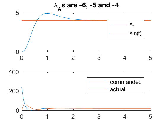
A = [0 1 0 0; 0 0 1 0;0 -5 -2 1; 0 0 0 -5];
B = [0 ;0 ;0;5];

p = [-3;-4;-5;-6];
K = place(A,B,p);
[v,d] = eig(A-B*K);

x_des = 4;

control = @(t,x)[-K*(x - [zeros(size(t));x_des*ones(size(t));zeros(size(t));3*x_des*ones(size(t))] )];
sys_dyn = @(t,x)[A*x + B*control(t,x)-[x_des;0;0;0] ];
Tspan = 0:0.02:5;
x0 = [0;0;0;0];

[t,x] = ode45(sys_dyn,Tspan,x0);
figure;
subplot(2,1,1)
plot(t,x(:,2),t,x_des*ones(size(t)))
legend('x_1','sin(t)')
title(['\lambda_As are ' num2str(d(1,1)) ', ' num2str(d(2,2)) ' and ' num2str(d(3,3))])
subplot(2,1,2)
plot(t',control(t',x'),t',x(:,4)')
legend('commanded','actual')

err2 = x(:,2)-sin(w*t);
%axis([0 25 -10 10])
max(x(:,4)')

Fig 8. - Pole-placement controller with actuator dynamics gives control signals much smaller in magnitude, and they start from 0.

A = [0 1 0 0; 0 0 1 0;0 -5 -2 1; 0 0 0 -5];
B = [0 ;0 ;0;5];

p = [-2;-3;-4;-10];
K = place(A,B,p);
[v,d] = eig(A-B*K);

w = 2;

control = @(t,x)[-K*(x - [zeros(size(t));sin(w*t);w*cos(w*t);-w^2*sin(w*t)+2*w*cos(w*t)+3*sin(w*t)] )];

sys_dyn = @(t,x)[A*x + B*control(t,x)-[sin(w*t);0;0;0] ];
Tspan = 0:0.1:20;
x0 = [0;0;0;0];

[t,x] = ode45(sys_dyn,Tspan,x0);
figure;
subplot(2,1,1)
plot(t,x(:,2),t,sin(w*t))
axis([0 20 -1 1])
legend('x_1','sin(t)')
title(['\lambda_As are ' num2str(d(1,1)) ', ' num2str(d(2,2)) ' and ' num2str(d(3,3))])
subplot(2,1,2)
plot(t',control(t',x'),t',x(:,4)')
legend('commanded','actual')

err2 = x(:,2)-sin(w*t);
%axis([0 25 -10 10])

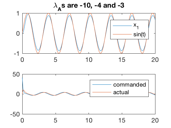
Fig 9. - Pole-placement controller with actuator dynamics gives control signals much smaller in magnitude, and they start from 0, which assuring good tracking performance.

Simulation results above indicate that by using actuator dynamics, a slightly poorer performance is achieved, however, the commanded control inputs are not large, and more importantly obey first order actuator dynamics.

Conclusions

In this session, we studied controllability, and went over applications of one pole-placement based controller synthesis method. By choosing the eigenvalues (poles) of the system carefully, it is possible to make the controller track a desired behavior. However, we havent discussed how to choose the appropriate eigenvalues, and the resulting controller gain matrix. In the next session, we will go over the concepts of optimaility and optimal control, and develop optimality conditions that can be used to derive gains for optimal control law.