Overview
- Vectors and vector operations
- Sum/difference
- Inner/outer products
- Matrix operations
- Eigen values and eigen vectors
- Singular value decompositions
- System of equations
- Matrix derivatives
- Least squares
Vectors
Vectors are scientific quantities that have both direction and magnitude. Vectors can be as simple as a line segment defined on a 2-D Euclidean plane, or a multi-dimensional collection of numerical quantities.
Sum/difference of vectors
Sum/difference of vectors is the vector of sum/differences
$$ \overrightarrow {a} = \left[ 1, 2, 3 \right] $$$$ \overrightarrow {b} = \left[ 3, 3, 4 \right] $$
$$ \overrightarrow {a}+\overrightarrow {b} = \left[ 1+3, 2+3, 3+4 \right] = \left[ 4, 5, 7 \right].$$$$ \overrightarrow {a}-\overrightarrow {b} = \left[ 1-3, 2-3, 3-4 \right] = \left[ -2, -1, -1 \right].$$Vector sum (or difference) is defined only between the vectors of the same dimension.
Inner Product
Inner product (also dot product) of two vectors \(\overrightarrow {a} \) and \( \overrightarrow {b}\) is defined as,
$$ \overrightarrow {a} \circ \overrightarrow {b} = \overrightarrow {a}^T \overrightarrow {b} = \sum_{i=1}^n a_i b_i, $$where \(n\) is the length of the vectors \(\overrightarrow {a} \) and \( \overrightarrow {b}\).
- Inner product represents how similar two vectors are to one another. This is also referred as Cosine similarity.
$$ cos(\theta) = \frac{\overrightarrow {a} \circ \overrightarrow {b}}{ | \overrightarrow {a}| |\overrightarrow {b}|} ,$$ - Inner product also represents the length of the projection of one vector along the other vector. Therefore, the projection of vector \(\overrightarrow {a}\) along vector \(\overrightarrow {b}\) is $$ \frac{\overrightarrow {a} \circ \overrightarrow {b}}{ |\overrightarrow {b}|} .$$
Inner product is defined only between the vectors of the same dimension.
Outer Product:
Outer product of two vector \( \overrightarrow {a} \) and \( \overrightarrow {b}\) is the matrix \(C_{ij}\) such that
$$ C_{ij} = a_i b_j$$Outer product is helpful in certain applications to reduce computation and storage requirements.
Outer product is defined between any two vectors and has no contraint on the length of either vector.
Matrices
A matrix (plural matrices) is a rectangular array of numbers, symbols, or expressions, arranged in rows and columns. In control systems, matrices are used to describe how the state vectors (for example position and velocity) evolve and how the control signal influences the state vectors. A matrix with \(n\) rows and \(m\) columns has a dimension of \( n \times m\) matrix and is represented as \(A_{n \times m}\) .
Sum/difference of matrices:
Sum/difference) of two matrices is equal to the matrix formed by sum (or difference) of individual elements, and has the same dimension as the original matrices. For example, sum of matrices \( A = a{i,j}\) and \( B = b{i,j}\) is
$$ C =c_{i,j} = a_{i,j} + b_{i,j} . $$Matrix sum (or difference) is defined only between the vectors of the same dimension.
Product of matrices:
Product of matrix and scalar
Product of a matrix with a scalar is equal to the matrix formed by multiplying each element of the matrix by the scalar. Therefore,
$$ \lambda A = \lambda a_{i,j} $$Product of matrix and matrix
Product of matrices , \( A B \) between two matrices $A_{n \times p}$ and $B_{p \times m} $ as,
$$ C_{n \times m} = A_{n \times p} B_{p \times m} = c_{i,j} = \sum_{k=1}^{p} a_{i,k} b_{k,j}, $$The matrix product is defined only if the number of columns in \(A\) is equal to the number of rows in \(B\). (\(C\)) is of dimension \( n \times m \).
Note: Outer product can also be used to compute matrix product, and typically results in lower computation and storage requirements.
$$ C_{n \times m} = \sum_{k=1}^{p} A_{(i,:)} B_{(:,j)}, $$Product of matrix and vector (column space or range)
Product of a matrix with a vector is defined in a similar manner as above, however in the special case of multiplying a matrix by vector results in linear combination of the columns.
$$ A_{n\times m} b_{m \times 1} = \left[ A_{(:,1)} A_{(:,2)} ... A_{(:,m)} \right] b_{m \times 1}$$Expanding \(b_{m \times 1}\) as \([b_1 b_2 ... b_m]^T\) and multiplying gives,
$$ A_{n\times m} b_{m \times 1} = b_1 A_{(:,1)}+ b_2 A_{(:,2)}+ ... + b_m A_{(:,m)} $$Therefore, the product of $ A_{n\times m}$ and $b_{m \times 1}$ is a linear combination of the columns of \(A\) and the weighing factors are determined by the vector $b_{m \times 1}$. The space spanned by the columns of \(A\) is also called the column space or range of the matrix \(A\).
Product of vector and matrix (row space)
Product of a vector with a matrix results in linear combination of the rows.
$$ a_{1\times n} B_{n \times m} = a_{1 \times n} \left[ \begin{array}{c} B_{(1,:)} \\ B_{(2,:)} \\ \vdots \\ B_{(n,:)} \\ \end{array} \right] $$Expanding \(a_{1 \times n}\) as \([a_1 a_2 ... a_n]\) and multiplying gives,
$$ a_{1\times n} B_{n \times m} = a_1 B_{(1,:)}+ a_2 B_{(2,:)}+ ... + a_n B_{(n,:)} $$Therefore, the product of $ a_{1\times n}$ and $B_{n \times m}$ is a linear combination of the rows of \(B\) and the weighing factors are determined by the vector \(a_{1 \times n}\). The space spanned by the rows of \(B\) is also called the row space or range of the matrix \(B\).
Rank of a matrix
The rank of the matrix is equal to the number of independent rows (or columns). Note, column and row ranks of a matrix are equal. Check the wikipage for a brief description of why.
c) Determinant of a matrices:
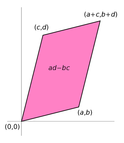
Determinant, defined for square matrices is an estimate of the 'size' of a matrix. Determinants represent the volume enclosed by the rows of the matrix in an n-dimensional hyperspace. For a 2-dimensional matrix, the determinant represents area enclosed by the vectors composed of the rows (or columns) of the matrix.
Inverse of matrices:
Inverse of a square matrix is the matrix that when multiplied by the original matrix gives an identity matrix. Identity matrix is a matrix that has 1s for diagonal terms and 0 for all the off-diagonal terms. Inverse of a matrix is computed as the matrix of cofactors divided by the determinant of the matrix, details here. Cofactors of an element \( i,j \) of a matrix is the matrix formed by removing \(i^{th} \) column and \(j^{th} \) column.
Matrix inverse example
Compute the inverse of
$$ A = \left[ \begin{array}{ccc} 1 & 2 & 3 \\ 4 & 5 & 6 \\ 7 & 8 & 1 \end{array} \right]$$Matrix inverse example
- Compute minors: Minor of an element at \( (i,j)\) position is taken by removing \( i^{th}\) row and \(j^{th}\) columns.
- Compute cofactor: Cofactor of an element at \( (i,j)\) position is taken by computing the Minor and then multiplying it with \( (-1)^{i*j} \)
- Compute inverse by replacing each element of the matrix by its cofactor and taking transpose.
Eigen values and eigen vectors:
Consider a vector \(\overrightarrow{v}\) such that
$$ A \overrightarrow{v} = \lambda \overrightarrow{v},$$i.e. product of the matrix \(A\) times the vector \(\overrightarrow{v}\) is the vector \(\overrightarrow{v}\) scaled by a factor of \(\lambda\). The vector \(\overrightarrow{v}\) is called the Eigen vector and the multiplier \(\lambda\) is called the eigen value. Eigen values are first computed by solving the characteristic equation of the matrix
$$ det( A - \lambda I) = 0, $$and next the first equation \( A \overrightarrow{v} = \lambda \overrightarrow{v}\) is used to obtain non-trival solution of eigen vectors. Eigen vectors are scaled so their magnitude is equal to 1.
If \(V\) is the matrix of all the eigen vectors then,
$$ AV = V \Lambda$$where \(\Lambda\) is the matrix whose off-diagonal terms are 0, and diagonal terms are eigen values corresponding to eigen vectors in the columns of \(V\). Therefore, \( A = V \Lambda V^{-1}\) or \(\Lambda = V^{-1} A V\). In the special case where \(V\) is unitary, \( A = V \Lambda V^T\) or \( \Lambda = V^T A V\).
Properties of eigen vectors and eigen values
- Eigen vectors are defined only for square matrices. For non-square matrices, singular value decomposition, or SVD is used.
- It is possible for a matrix to have repeated eigen values.
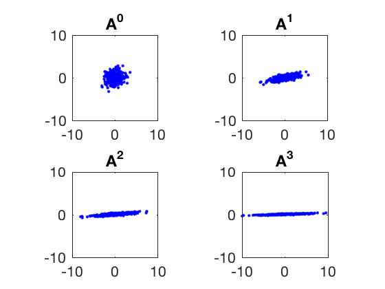
- Matrix multiplication transforms data in such a way that directions along larger eigen values are magnified.
- The space spanned by all the eigen vectors whose eigen values are non-zero is also the column space of the matrix.
- If an eigen value is 0, then its corresponding eigen vector is called a null vector. The space spanned by all the null vectors is called the null space of the matrix.
- If any of the eigen values is equal to 0, the matrix is not full rank. Infact, the rank of a square matrix is equal to the number of non-zero eigen values.
- The determinant of a matrix is equal to product of the eigen values.
- Eigen values represent how much the data will get skewed by multiplying it with the matrix A. The eigen vectors corresponding to largest eigen value become dominant while the smaller eigen values' vectors diminish.
Eigen value example
Consider the matrix,
$$ A = \left[ \begin{array}{ccc} 1.5 & 1 \\ 0 & 0.5 \end{array} \right]$$- Find eigen values of A
- What will happen to a vector when it is multiplied by \( A \)?
Eigen value example
$$ A = \left[ \begin{array}{ccc} 1.5 & 1 \\ 0 & 0.5 \end{array} \right]$$- Find eigen values of A, 0.5 and 1.5
- What will happen to a vector when it is multiplied by \( A \)?
Properties of eigen values and eigen vectors.
- Trace of a matrix (sum of all diagonal elements) is equal to the sum of eigen values
- Determinant of a matrix is equal to the product of eigen values.
- A set of eigenvectors of \(A\), each corresponding to a different eigenvalue of \(A\), is a linearly independent set.
- A matrix is positive (or negative) definite if all its eigen values are either positive (or negative).
Singular value decomposition (SVD)
Singular value decomposition or SVD is a powerful matrix factorization or decomposition technique. In SVD, a \( n \times m\) matrix \(A\) is decomposed as \( U \Sigma V^{*} \),
$$ A = U \Sigma V^{\*} $$where \(U\), \( \Sigma \) and \( V \) satisfy
- \( U \) is called the matrix of left singular vector, and its columns are eigen vectors of \( A A^{*} \).
- \( V \) is called the matrix of right singular vector, and its columns are eigen vectors of \( A^{*} A \).
- \( \Sigma \) is a \(n \times m \) matrix whose diagonal elements are square root of eigen values of \( A A^{*} \) or \( A^{*} A \).
- For most matrices \( n \neq m \), therefore, the maximum rank \(A\) can have is the lower of \( m \) or \( n \).
- If \( n > m \), then \(A \) has more rows than columns and \( \Sigma \) is a matrix of size \( n \times m \) and its \( i,i \) element is square root of eigen value of \( A A^{*} \) or \( A^{*} A \) for \( i = 1\) to \(m\).
- If \( n < m \), then \(A \) has more columns than rows and \( \Sigma \) is a matrix of size \( n \times m \) and its \( i,i \) element is square root of eigen value of \( A A^{*} \) or \( A^{*} A \) for \( i = 1\) to \(n\).
Note: \( V^{*} \) is complex conjugate of \(V\). If all elements of \(V\) are real then \(V^{*} = V^T\).
Applications of SVD
SVD is a powerful dimensionality reduction technique.
The eigen vectors of covariance matrix also represent the percentage of explained variance in data.
- Therefore, square of singular values of a matrix represent the relative amount of data explained by the corresponding eigen vector.
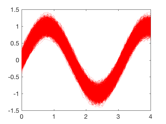
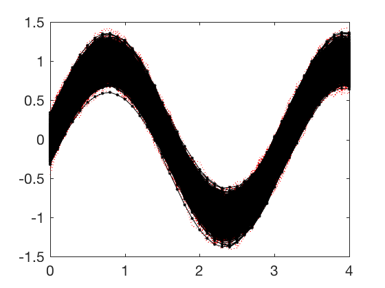
SVD example 1
Raw_signals reconstructed using first 4 components, see notes for code and implementation details. Savings of 90% in storage by losing 1% accuracy.
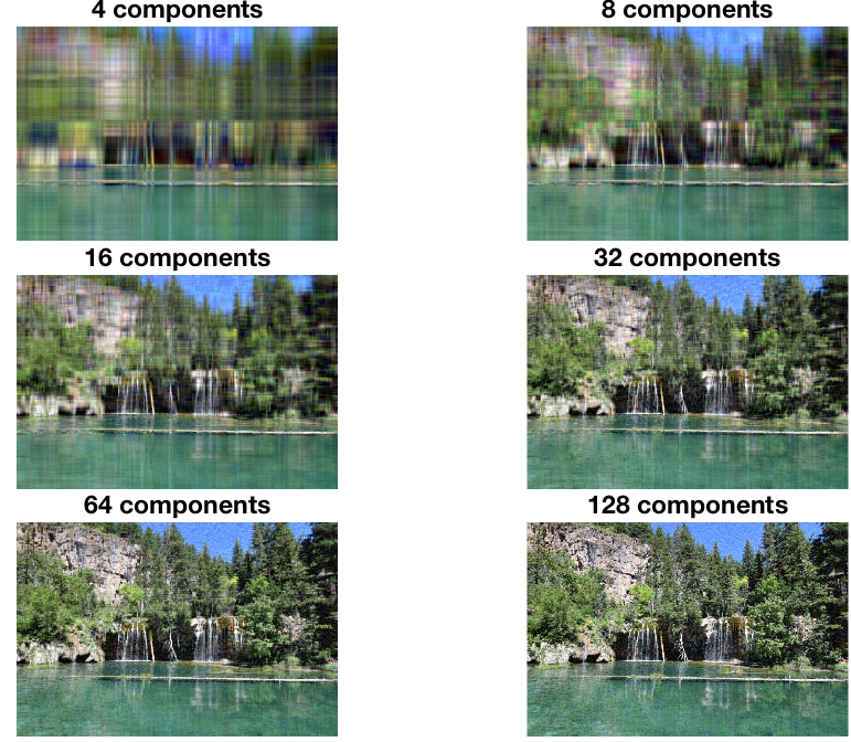
SVD example 2
SVD for image compression. SVD can be used for image compression too.
- Images are matrix of numbers
- Images typically have many correlated features.
- Images of size $N \times N$ have storage requirement of $N^2$
- If you take selected few components, the storage requirements drop.

SVD example 2
Systems of equation
In control theory, we often come across equations of the form $ A_{n \times m} x_{m \times 1} = b_{n \times 1} $ where given \(A\) and \(b\), we wish to solve for \(x\). Lets consider the following cases,
- When \(n = m \), in this case the matrix \(A\) is a square matrix and a unique solution \( x = A^{-1} b \) exists if \( A\) is full rank. If \(A\) is not full rank, then no solutions exist if \(b\) has a component along the null space of \(A\).
- When \(n > m \), in this case, there are more equations (or constraints) than free parameters. Therefore, it is not possible to find a solution that solves \( A x = b\) for any \( x \). Such equations typically arise when we want to estimate some parameter from multiple observations. A typical approcah to solve such type of equations is to formulate an error function (sum of squared errors), and find parameters that minimize it.
- When \(m > n \), in this case, there are more unknowns than equations, and solution exists if rank of \(A\) is equal to \(n\). If \(A\) is not full rank, then \(Ax\) cannot have components along null space of \(A\). Therefore, if \(b\) has a component along null space of \(A\) then solutions do not exist. These types of equations are very common in control synthesis, where there are multiple ways to control the same system to achieve the same goal. Typically controller parameters are varied to minimize certain cost that combines task and control effort.
Least square fitting
Problem statement
Given a set of \( N \) training points such that for each \( i \in [0,N] \), \( \mathbf{x}_i \in R^M \) maps to a scalar output \(y_i\), the goal is to find a linear vector \(\mathbf{a}\) such that the error
$$ J \left(\mathbf{a},a_0 \right) = \frac{1}{2} \sum_{i}^{N} \sum_{j}^{m} \left( a_j x_{i,j} + a_0 - y_i \right)^2 , $$is minimized. Where \(a_j \) is the \( j^{th} \) component and \( a_0 \) is the intercept.
Sum of squared errors
The cost fuction above can be rewritten as a dot product of the error vector
$$ e(W) = \left( X W - y \right) .$$where X is a matrix of n times m+1, y is a n-dimensional vector and W is (m+1)-dimensional vector.
Therefore, the cost function J is now,
$$ J \left(\mathbf{W} \right) = \frac{1}{2} e(W)^T e(W)= \frac{1}{2} \left( \mathbf{ X W - y } \right)^T \left(\mathbf{ X W - y } \right) .$$After some matrix derivatives
Expanding the transpose term, $$ J \left(\mathbf{W} \right) = \frac{1}{2} \left( \mathbf{W^T X^T - y^T} \right) \left(\mathbf{ X W - y }\right) $$
$$ = \frac{1}{2} \left( \mathbf{ W^T X^T X W - 2 y^T X W + y^T y} \right) $$Note, all terms in the equation above are scalar. Taking derivative with respect to W gives,
$$ \frac{\partial \mathbf{J}}{\partial \mathbf{W}} = \left( \mathbf{ W^T X^T X - y^T X } \right) $$Gradient-descent method
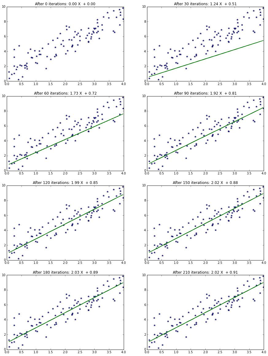
Minimum is obtained when the derivative above is zero. Most commonly used approach is a gradient descent based solution where we start with some initial guess for W, and update it as,
$$ \mathbf{W_{k+1}} = \mathbf{W_{k}} - \mu \frac{\partial \mathbf{J}}{\partial \mathbf{W}} $$It always a good idea to test if the analytically computed derivative is correct, this is done by using the central difference method, $$ \frac{\partial \mathbf{J}}{\partial \mathbf{W}}_{numerical} \approx \frac{\mathbf{J(W+h) - J(W-h)}}{2h} $$
Central difference method is better suited because the central difference method has error of \( O(h^2 \), while the forward difference has error of \( O(h) \). Interested readers may look up Taylor series expansion or may choose to wait for a later post.
Gradient-descent method
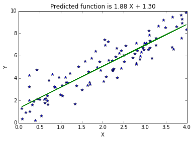
Pseudoinverse method
Another method is to directly compute the best solution by setting the first derivative of the cost function to zero.
$$ \frac{\partial \mathbf{J}}{\partial \mathbf{W}} = \left( \mathbf{ W^T X^T X - y^T X } \right) = \mathbf{0}$$By taking transpose and solving for W,
$$ \mathbf{W} = \mathbf{ \underbrace{(X^T X)^{-1}X^T}_{Pseudoinverse} ~ y } $$Pseudoinverse method
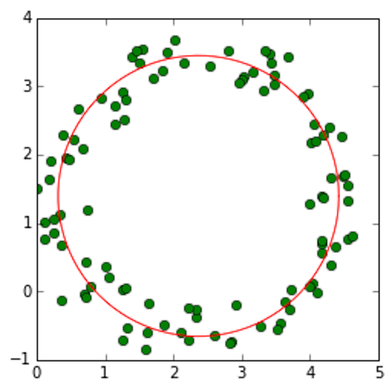
Circle fitting
Conclusion
- Vector and matrix definitions
- Inner and outer products
- Ranks and determinants
- SVD and eigen value problems