Welcome
Welcome to the homepage of MEC 560: Advanced control systems offered at Stony Brook University and taught by Dr Vivek Yadav. If you have any questions, feedback, concerns or spot any items that need correction, please email Dr Vivek Yadav directly.
Control systems overview
A control system is a device, or set of devices, that manages, commands, directs or regulates the behaviour of other devices or systems. Industrial control systems are used in industrial production for controlling equipment or machines. From wikipedia. This definition although accurate is not detailed. In this couse, we will develop a more detailed understanding of what control system is, and challenged associated with designing an real-world ready controller.
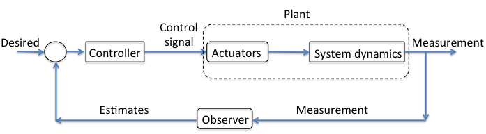
Consider the example of maintining the speed of the car using cruise control. This typically involves 'measuring' the speed of the car, computing throttle opening/closing based on deviation from the desired speed, and applying this control signal to the car's throttle. This process can be better understood by separating the involved concepts into 4 parts, plant, measurement and estimation, control law and actuation. These are discussed in more detail below,
Plant: Plant is the physical system that we want to behave in a certain manner. Plant is the system that we interact with using control signals applied via actuators and whose state we monitor using estimates derived from sensors measurements. We define states of a system as the variables that specify the system. In our example, position, orientation and their velocities form the states of the car. Note, the constants required to accurately describe the system are called parameters, for example mass of the car, wheel diameter, throttle bandwidth, etc. The states of a system are not unique.
Observer (Measurements and estimation): Observers are used to convert measurements into state estimates. In our example, to precisely control the speed of the car, we first need to get the speed of the car relative to the ground. However, the speed of the car is not directly measured. Speed is typically estimated by measuring the rotational speed of the drive shaft, and using a calibration table to convert the drive shaft's rotational speed to the speed of the car. This technique is prone to errors due to sensor noise, differential wear of tires, road conditions, etc. The observer design deals with how to best estimate the ground speed of the car given the measurements of the rotational speed of the drive shaft. Where as estimation deals with how to best estimate the speed of the car from the position of the car. Estimates can futher be improved by combining measurements from multiple sensors. For example, most modern cars are equipped with a GPS, therefore estimates of speed can be improved by combining data from GPS and drive shaft. This process is also refered to as sensor fusion. Kalman filters are often used for sensor fusion.
Actuation : Actuators are devices that interact with a plant and change its inherent states. States are defined as variables that are required to uniquely define what the plant is doing. For example, for a car, the states are location on the road, heading, rate of change of location on the road and rate of change of heading. In our cruise control example, throttle is the actuator whose opening is adusted to vary the speed of the car. Consider a simple control law where we compute the difference between the desired and estimated speed as command to the throttle. Therefore, if desired speed is lower than the estimated speed, the difference is positive and throttle is asked to open. If the desired speed is lower than the estimated speed, the difference is negative and the throttle is asked to let lesser fuel in. However, there are physical limitations on how much the throttle can open or close. The throttle opening cannot be more than the diameter of the inlet fuel line and closing cannot be lower than 0. These constraints also called 'actuator constraints' dictate how we may interact with a system. Further, any actuation system cannot directly apply the commanded control, and there is a lag in response. This lag is response is also called 'actuator dynamics'. Actuator dynamics are difficult to estimate as they depend on multiple factors, they are usually modeled as a first order decay system.
Control law : Control law is the law that governs how the estimates are converted to signals to be sent to the actuators. One way to obtain control signal is to compute the difference between the desired and actual states of the system and scaling them up by appropriate gain factors (refered to as proportional, integral or derivative or PID control). The resulting control signal is sent to the actuator. It is important to have an actuator with large bandwidth because a less responsive actuator can severely affect the performance of the controller. Note, bandwidth is the frequency at which the corresponding frequency response has an amplitude of -3dB and phase difference of 180. Also, bandwidth is related to time constant via $f_{3dB} = \frac{1}{2 \pi \tau}$. Therefore, larger bandwidth implies smaller time constant and thus faster response. Systems in which the control is based on all the states of the system is called full state feedback. However, it is not always possible to have full state feedback, for example, in cruise control example, we are not interested in actual position of the car, only the velocity. As we will learn later, PID control can be achieved by using infinitely many combinations of the underlying gains. However, most PID control systems do not explicitly account for system dynamics, therefore, are not efficient. An efficient controller can be synthesized using a detailed model of the system. The field of control theory that deals with designing such optimal control laws is called optimal control theory. Optimal control laws explicitely consider the system dynamics and give control law that best minimizes some cost objective that typically weighs deviation from the desired states and the involved control effort. However, such models are prone to errors due to inaccurate estimation of system dynamics and its corresponding parameters. For example, the mathematical model describing an airplane has drag coefficients, and these coefficients vary with wind conditions. Further, mass or inertia of the airplane may change due to payload, cargo load or other factors. As evident, control laws are susceptible to errors due to errors in estimating model parameters, inaccurate/incomplete system dynamics model, sensor and actuation noise, actuator contraints and actuator dynamics. The field of control theory that deals with synthesizing controllers for systems operating under uncertain conditions is robust control.
Course Topics:
This course specifically deals with item 4 above. We will learn techniques to to obtain the best control law that guarantees stability, low tracking error and optimality. We will specifically study control systems using the state space formulation, primers on related concepts will be provided as and when needed.
- Linear system theory: state-space model and its solution, stability, controllability, observability, pole placement, state observers, and observer-based compensators We will spend a lot of time studying linear systems because mathematical techniques have been developed that ensure stability of the control law, let us determine if a system is controllable and observable, provide computational framework to choose a good control law, design state observers and apply observer-based control. These computational frameworks provide a systematic approach to analyzing dynamic systems. Although, they are developed for linear systems, they can easily be extended to nonlinear systems, which we will do in the third phase of this course.
- Optimal and robust control: system norms and performances, linear quadratic control and Kalman filter, H-infinity control. This section deals with the development of control laws, optimal obervers and robust control design. The mathematical concepts from the previous sections will be applied to design control laws. The most common task in designing control law is to choose gains on error terms, however choosing large gains can result in a control system that is very reactive. This involves wastage of control effort and may damage the actuator. On the other end is a control system that has very low gains. Although lower gains ensure low control cost and minimal risk to actuators, they usually result in poorer performance. Therefore, there is a trade off between controller's performance and control effort, and optimization techniques are applied to select the appropriate gain factors. Similarly, while designing control law for a real-world application, there is always a chance that the modeled dynamics is not complete or the model parameters are not known. For such applications, H-infinity type of control is developed which guarantees stable control with certain minimum performance.
- Introduction to nonlinear systems analysis, Lyapunov methods, sliding and adaptive controls. This section extends the ideas developed in the previous lessons to non-linear systems. In particular, we will learn how to linearize a non-linear system, and apply linear control laws. Linearization is efficient if the linearization error (error between linear form and actual nonlinear system) is small, therefore researchers have proposed other techniques such as nonlinearity cancelation, state-dependent ricatti equation, etc. Techniques to analyze and control nonlinear systems will be presented and applied for this part of the course.
- Special topics, neural networks based control, model predictive control, reinforcement learning for control, (approximate) dynamic programming. All the above methods involve accurately modeling the system dynamics, even the robust control methods require the user to input how the underlying disturbance affects the system dynamics. Therefore, for real-world applications these techniques are not fully applicable and often result in poorer than promised performance. Many concepts from the emerging field of machine learning or artificial intelligence can be applied to design more robust control laws. The last part of the course will provide introduction to these emerging ideas and students are encouraged to use them in their course projects.
Recent Notes:
-
Nov 22, 2016
Lyapunov methods
Lyapunov methods . -
Nov 22, 2016
Linearization: Nonlinear Dynamic Inversion, (input-output) Feedback Linearization and input-state linearization (SISO only)
Linearization: Nonlinear Dynamic Inversion, (input-output) Feedback Linearization and input-state linearization (SISO only). -
Nov 4, 2016
Applying principles of linear control systems for control of nonlinear system dynamics
Applying principles of linear control systems for control of nonlinear system dynamics. -
Oct 29, 2016
Kalman filter
Kalman filtering and estimation for linear systems. -
Oct 14, 2016
Control and estimation under uncertainity
Control and estimation under uncertainity -
Oct 1, 2016
Output feedback control, Observability and Observer design
Output feedback control, observability and full-order/reduced-order observer design for linear systems using pole-placement. -
Oct 1, 2016
Nonlinear control systems: Introduction and Analysis
Nonlinear control systems: Introduction and Analysis. -
Sep 30, 2016
Direct collocation for optimal control
Direct collocation for optimal control, GPOPs II. -
Sep 25, 2016
Optimal control
Optimal control concepts, LQR, Multiple shooting, HJB equations. -
Sep 19, 2016
Controllability
Derivation of controllability conditions for a linear system dynamics. -
Sep 19, 2016
Control synthesis
Control synthesis, pole-placement for control of spring mass damper system under different conditions. -
Sep 11, 2016
System dynamics and State-space Representations
System dynamics and State-space Representations. -
Sep 11, 2016
Solution of linear differential equations in state space form
Solution of state space models and their properties. -
Aug 30, 2016
Deriving equations of motion for a 2-R manipulator using MATLAB
Lagrange methods to derive equations of motion of robotic systems under no contraints is presented. MATLAB scripts are provided that implement that perform same calculations using symbolic toolbox. -
Aug 29, 2016
Linear Algebra review
Review of the required linear algebra concepts for control systems theory. -
Aug 29, 2016
Least-square fitting using matrix derivatives
Matrix differentials and their applications for getting least-square curve fits. -
Aug 29, 2016
Control systems overview
Introduction to control systems design and the scope of MEC 560.